Backtesting Stochastic Oscillator Settings: Step-by-Step

Backtest a stochastic strategy by defining the trades first, then comparing settings under the same data and execution assumptions. A better-looking oscillator or a higher win rate is not enough. The test must include exits, position sizing, costs and a period that was not used to select the parameters.
On LuxAlgo’s native charts, Quant, our coding agent, can help turn those written rules into a strategy you can inspect and run. Start with a baseline, review individual trades, and change only what the experiment is intended to measure.
Step 1: Name the Inputs and Choose One Signal
The raw stochastic value is the close’s position within a recent high–low range, scaled by 100. In a smoothed implementation, %K averages that value and %D averages %K. TradingView’s stochastic documentation separates the range period, %K smoothing and %D period.
| Candidate | Range lookback | %K smoothing | %D period |
|---|---|---|---|
| Baseline | 14 | 3 | 3 |
| Shorter-window example | 9 | 2 | 3 |
| Longer-window example | 21 | 3 | 5 |
The named inputs remove the ambiguity in tuples such as 9-3-2 and 21-5-3. These examples are not proven recommendations for particular chart intervals. Fast, slow and full stochastic refer to constructions and available controls, rather than three universal numerical presets.
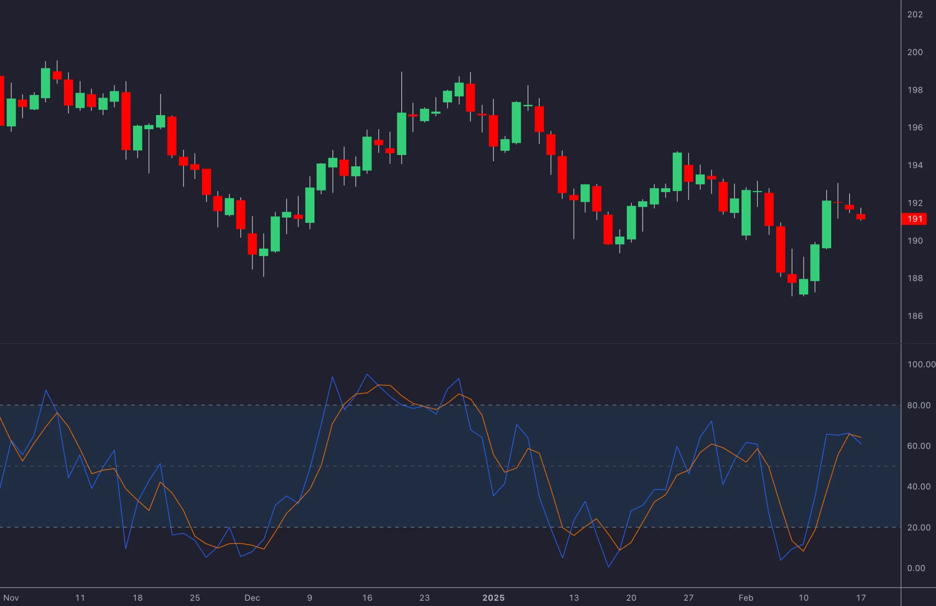
Choose the signal you will test before varying settings:
- Extreme-zone exit: %K moves from at or below 20 to above 20. This differs from merely remaining oversold.
- %K/%D crossover: %K crosses above %D. Specify whether an extreme-zone filter is also required.
- Centerline crossover: %K crosses above 50. This is a different event, not confirmation of every other signal.
- Divergence: define the paired swings, oscillator series and pivot-confirmation delay. A historical pivot cannot be used before it becomes known.
For a simple baseline, test long entry after a completed %K/%D bullish crossover and exit after a completed bearish crossover. This intentionally isolates the crossover rule. Any stop, target, trend filter or 80/20 restriction creates a different variant that should be documented.
Step 2: Specify Data, Dates and Execution
Record the symbol and venue, chart interval, session, data source and test dates. Use standard market-price candles for fill testing. Synthetic candle prices, such as Heikin Ashi values, can produce trades at prices that were not available.
One or two years may be a starting sample, but it is not universally sufficient. A monthly strategy may generate very few trades over that period, while an intraday strategy may encounter thousands of correlated observations. Include different conditions and allow enough earlier bars for indicator warm-up.
Check missing or duplicate bars, timezone alignment and corporate-action treatment. For equities, use consistent split adjustment and decide how dividends are represented; do not combine adjusted closes with incompatible raw highs and lows. Futures rolls, expired contracts and changing stock universes also need explicit treatment where relevant.
| Assumption | What to record |
|---|---|
| Orders and fills | Signal timing, next-bar or other fill policy, order type and unfilled-order treatment |
| Costs | Commission, spread/slippage assumptions, and any relevant financing or borrowing costs |
| Capital | Initial equity, position size, margin and pyramiding policy |
| Open positions | How positions remaining at the end of the test are reported |
| Validation | Development dates, selection rules and separate evaluation dates |
Use a consistent accounting policy across variants. A strategy with small average trades can lose its apparent advantage after realistic costs. A percentage allocation is the capital committed to a position, not a guaranteed percentage loss limit.
Step 3: Build and Inspect the Native Quant Test
Describe the oscillator inputs, crossover rule, exits, sizing and costs to Quant. Review the code and plotted signals before interpreting the return. Ask it to resolve missing assumptions explicitly rather than infer your intended strategy from “find the best stochastic settings.”
In the native strategy workflow, Run executes a strategy on the chart’s history. The summary displays net profit, closed trades, win rate, maximum drawdown and profit factor. Open the viewer for Performance, Trades Analysis and Trades Log.
Use Inputs for exposed strategy parameters and Properties for capital, order size, pyramiding, commission, slippage and margin. Inspect entries and exits against the written rule. Star a run to retain its script, symbol, timeframe, inputs and backtest properties.
Start by finding several entries, exits and periods with no trade. Check that a crossover is a one-bar event, that the position closes under the intended condition, and that historical higher-timeframe or divergence information is not used early. Correct syntax does not prove correct strategy logic.
Step 4: Use a Complete TradingView Example When Comparing Platforms
For readers testing the same baseline in TradingView, the example below shows the full calculation and order rules in Pine Script® v6. The documented ta.stoch call takes the source, high, low and range length and returns one series. Smooth that series to obtain %K, then calculate %D separately.
This teaching strategy is long-only, enters on a completed bullish crossover and exits on a bearish one. It has no extreme-zone filter, stop-loss or profit target. Its 10% equity allocation, 0.05% commission per filled order and one-tick slippage are illustrative simulation assumptions to replace for your market.
//@version=6
strategy("Stochastic crossover baseline", overlay=false,
    initial_capital=10000,
    default_qty_type=strategy.percent_of_equity,
    default_qty_value=10, pyramiding=0,
    commission_type=strategy.commission.percent,
    commission_value=0.05, slippage=1,
    process_orders_on_close=false)

kLength = input.int(14, "Range lookback", minval=1)
smoothK = input.int(3, "%K smoothing", minval=1)
dLength = input.int(3, "%D period", minval=1)

rawK = ta.stoch(close, high, low, kLength)
k = ta.sma(rawK, smoothK)
d = ta.sma(k, dLength)

enterLong = ta.crossover(k, d)
exitLong = ta.crossunder(k, d)

if enterLong and strategy.position_size == 0
    strategy.entry("Long", strategy.long)
if exitLong and strategy.position_size > 0
    strategy.close("Long")

plot(k, "%K", color=color.blue)
plot(d, "%D", color=color.orange)
hline(80, "Upper reference")
hline(20, "Lower reference")
Under TradingView’s default historical strategy behavior, calculations occur at bar close and market orders normally fill at the next bar’s open. The strategy documentation explains the broker emulator and cost settings. The 80/20 lines in this example are visual references; they do not restrict entries.
The example uses the available chart history and does not impose a date window or force liquidation at the last bar. Set matching test windows and accounting rules when comparing results. An open position is not the same as a closed trade, and differences in feeds, sessions or fill models can explain different platform results.
TradingView needs a strategy script with order logic for automated backtesting; adding an indicator alone does not create trades. Backtrader is an alternative Python framework for a custom research workflow, with data feeds, order handling, analyzers and optimization facilities. Its setup and data choices require programming; it is not an identical execution environment to native LuxAlgo charts.
Step 5: Compare Outcomes Before Tuning Parameters
Keep an experiment log with a version ID, dates, market, interval, inputs, rules and cost assumptions. Record net results, drawdown, number of trades and the distribution of wins and losses. Inspect timestamps, entry and exit prices, holding periods and any unusual fills.
There is no universal pass mark of 55% win rate, 1.5 profit factor or 1.5 Sharpe ratio. A high win rate can coexist with large losses, and a strong ratio from a small sample may be unstable. Profit factor is gross profit divided by gross loss; check how the report includes costs and handles periods with no losing trades.
For example, a hypothetical strategy winning 60% of trades with an average $8 win and $10 loss has an average outcome of 0.60 × $8 − 0.40 × $10 = $0.80 before costs. If round-trip costs average $1.20, its net expectation is −$0.40 per trade despite the 60% win rate.
If using Sharpe ratio in a separate analysis, keep the return frequency, annualization, risk-free-rate convention and treatment of idle capital consistent. Do not assume a metric is present in every platform’s report. Compare with a benchmark using the same dates and a meaningful exposure assumption.
Step 6: Change Settings as Controlled Experiments
First isolate a change to range lookback, smoothing or the entry threshold. A complete preset comparison changes several controls together and cannot tell you which one caused the difference.
Examples worth testing include longer lookbacks of 21–34 versus a 14-bar baseline, or shorter values of 5–9. A %D period of 2 versus 5–7 changes smoothing; thresholds of 70/30 versus 90/10 change the condition’s selectivity. None is automatically correct for a ranging or trending market.
Classify regimes using information available at the time if regime-specific rules are part of the strategy. Avoid labeling the entire period “trending” only after seeing its final path. Adding a trend or volume filter is another experiment and should be compared with the unfiltered baseline.
Look for nearby settings producing broadly similar behavior rather than a single isolated peak. Track every attempted configuration so you know how much selection occurred. Quant can help implement comparisons, but a visually appealing result does not prove that automated optimization found a durable advantage.
Step 7: Validate the Chosen Rules on New Periods
Reserve an evaluation period before choosing parameters. After selecting a configuration on development data, freeze it and assess that separate period. Repeatedly checking the evaluation set while retuning turns it into more development data.
A walk-forward design repeats this process through time: choose settings on an earlier window, apply them to the following unseen window, then advance the windows. Specify their lengths, selection rule, costs and how positions crossing boundaries are handled. Do not assume a platform performs walk-forward analysis merely because it runs a standard historical backtest.
Test other suitable instruments and different cost assumptions, then paper trade the workflow. Results should be interpreted alongside sample size, changing market conditions and execution constraints. Use the LuxAlgo Journal to review recorded trades and notes; keep the research configurations in your experiment log.
A useful outcome is a reproducible rule whose strengths and limits you can explain. A parameter set that wins the historical ranking is a candidate for further evaluation, not a guarantee of future returns.
Read next