Mean Reversion Playbook - Fade, Scale, Exit
A mean-reversion trade fades a move away from a defined reference and looks for a return toward it. The reference might be a rolling moving average, session VWAP or a modeled spread. Price is not obliged to return, and the reference itself can move while the trade is open.
This playbook connects three decisions: when to fade, how much exposure to take and how to scale out. Use LuxAlgo’s charting and AI platform to inspect the setup on Quant Charts, then work with Quant, our coding agent, to implement explicit entries, partial exits and risk rules for testing.
- Define the mean: specify the calculation, window, price source and session reset.
- Define the trigger: an extreme reading alone is different from a completed recovery back inside a band.
- Budget the whole trade: include planned additions, remaining exposure and realistic stop execution.
- Compare exit models: scaling out reduces exposure but can also reduce the payoff from the largest winners.
Finding Mean-Reversion Trade Setups
Measure a Deviation Without Inventing a Probability
A simple standardized deviation is z = (price − mean) / standard deviation, provided the denominator is nonzero. Record whether the current candle is included in the calculation and whether the estimate is based on prices, returns or a spread; these are not interchangeable statistical objects.
For example, a price of $96 against a $100 rolling mean and a $2 standard deviation gives z = −2. That identifies a two-standard-deviation distance under the chosen calculation. It does not mean a reversal has a known probability or that $100 is a fixed destination.
Bollinger Bands commonly use a 20-period simple moving average with bands two standard deviations away. John Bollinger’s own rules stress that band touches are not standalone buy or sell signals, prices can move along a band during trends, and standard deviation does not justify normal-distribution assumptions about security prices.
A 1.5-standard-deviation threshold is another parameter to evaluate, not a universal statistical significance test. Changing the window, band width or mean changes which events qualify. An average that falls toward a losing long position can create an apparent “return to the mean” without producing the expected profit.
Use Complementary Evidence
| Measure | Useful question | Limitation to retain |
|---|---|---|
| Bollinger Bands or a z-score | How far is price from the chosen rolling reference? | An extreme can persist or expand |
| RSI | How does recent upward movement compare with downward movement? | Above 70 or below 30 does not force a reversal |
| MACD or oscillator divergence | Is momentum confirming the new price extreme? | Divergence can repeat throughout a strong trend |
| Volume and price structure | Is there a defined rejection, reclaim or change in participation? | A single volume bar does not prove exhaustion |
| Higher-timeframe context | Does the local fade oppose a larger directional move? | Use only information available at the entry time |
Do not rank Bollinger Bands plus RSI as automatically “high strength” or multiple-timeframe RSI as “very high strength.” Several indicators can encode related price information. Measure whether each added condition improves the chosen strategy after costs and missed trades.
The StockCharts RSI guide documents how overbought and oversold readings can persist in trends. A long candidate could require RSI to recover above 30, rather than buying merely because it is below 30. Those are separate models with different timing.
Distinguish Regular and Hidden Divergence
| Divergence | Price comparison | Oscillator comparison | Typical interpretation |
|---|---|---|---|
| Regular bullish | Lower low | Higher low | Possible weakening of downward momentum |
| Regular bearish | Higher high | Lower high | Possible weakening of upward momentum |
| Hidden bullish | Higher low | Lower low | Possible uptrend continuation |
| Hidden bearish | Lower high | Higher high | Possible downtrend continuation |
Hidden divergence is commonly a continuation concept, so it should not be treated as interchangeable with a countertrend fade. For any divergence, define the pivot rule, lookback and confirmation delay. A pivot requiring later candles was not knowable at its plotted turning point.
Consider a hypothetical Bitcoin sequence with a lower price low near $81,256 and a higher RSI low. That can define a regular bullish divergence candidate, but the oscillator values, timeframe and entry trigger are still needed. A later price above $87,000 would not show whether an earlier stop was hit or whether the strategy captured the move.
Likewise, a hypothetical EUR/USD sequence making higher highs near 1.05322 while RSI makes lower highs illustrates regular bearish divergence. A subsequent move below 1.04000 would need a dated, reproducible record before it could be cited as evidence. These examples are schematic; they are not verified April 2025 trades.
A reported S&P 500 profit factor of 1.75 across 2–20-day holding periods is not sufficient evidence without the rules, sample, trade count and costs. Divergence is a condition to test, not a guaranteed source of mean reversion.
Fade Entry Methods
Write the Setup and Trigger Separately
One research model could define an oversold setup as a completed close below the lower Bollinger Band. Its long trigger could require the next qualifying close back inside the band, with RSI recovering above a specified threshold. Entering outside the band, on the recovery close or at the next bar’s open creates three different execution models.
- Choose the regime. Define when fading is allowed and when trend or event conditions exclude it.
- Measure the extension. Specify the mean, deviation estimate and threshold, such as z below −2.
- Require the chosen response. For example, a completed band re-entry, a reclaim of a prior level or a confirmed divergence.
- Set invalidation and expiry. State the stop, maximum setup age and maximum holding time.
- Check actual-entry reward. Compare the fill with the intended mean target after spread and costs.
A declining-volume rule is optional evidence, not a requirement that defines every valid fade. Capitulation-style activity and quiet pullbacks are different hypotheses. Keep the volume feed and session consistent, and do not infer volume confirmation when the data are absent.
For shorts, reverse the directional conditions only where that is economically appropriate. Borrow costs, short-sale restrictions, asymmetric equity behavior and derivatives funding mean a mirrored rule may produce different results.
Scale In Only Within a Fixed Plan
Scaling into a position means adding exposure. Scaling out means reducing it. Gradual entries do not automatically reduce risk, especially when additions occur as the market moves against the first fill.
Suppose a predefined plan buys 100 shares at $98 and another 100 at $96, with a common $94 stop. The first tranche risks $400 and the second $200, for $600 of planned price risk before costs. The average entry becomes $97 across 200 shares. A better average price has not eliminated the exposure.
If the trade budget were only $400, that second tranche would exceed it unless other conditions changed within the original plan. Cap the total size, number of additions and worst planned loss in advance. Do not widen a stop or add indefinitely to rescue a failed mean-reversion premise.
Check Whether the Market Is Rotating or Trending
Repeated crossings around an average can support a rotational hypothesis. Persistent trading on one side of a sloping reference can support a trend hypothesis. These descriptions can change during a session, so any filter must use contemporaneous evidence rather than the day’s final classification.
Scheduled announcements, earnings gaps and thin liquidity can make a recent mean a poor reference. A broad market-breadth thrust, including a Zweig-style measure, answers a market-participation question; it is not a substitute for an individual instrument’s fade trigger. Specify the breadth universe and calculation before adding it to a model.
Analyze the Setup with LuxAlgo
Inspect Native VWAP Regimes on Quant Charts
The current VWAP Mean-reversion vs Trend Regimes Library indicator evaluates intraday behavior using crossings, side hold, VWAP slope and average stretch. Its composite score classifies rotational versus trending conditions; it is not a probability of the next trade winning.
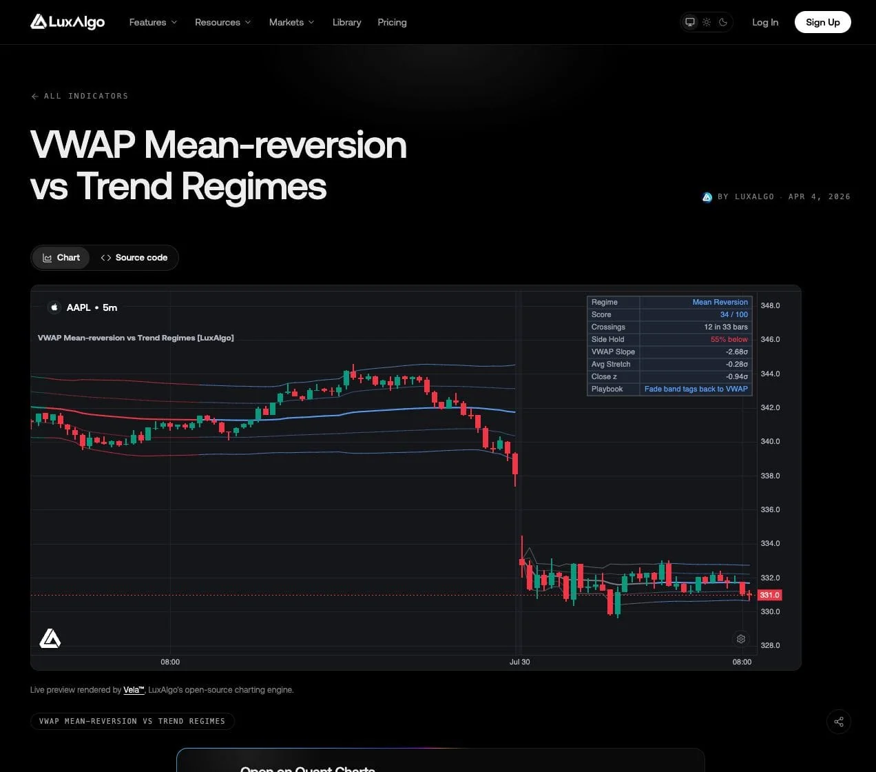
Documented defaults use a 48-bar evidence window with at least 12 bars before committing, a trend threshold of 65 and a mean-reversion threshold of 35. Between the thresholds, the previous classification is retained. The first and outer bands default to one and two volume-weighted deviations.
The indicator distinguishes a developing session from a committed regime and can reclassify as the evidence changes. Optional setup markers and regime-flip labels are off by default. Review the current inputs and source before interpreting a screenshot or comparing it with another VWAP implementation.
Use its Open on Quant Charts action to inspect it on Quant Charts. This is an intraday session-VWAP tool, not the same calculation as rolling Bollinger Bands. Keep the session reset and timeframe visible when comparing fade setups.
Scale-Out Exit Techniques
Allocate Percentages That Add Up
A scale-out plan might sell 35% of the original position at the chosen mean, another 35% at a second objective and the final 30% under a runner rule. These percentages add to 100%; ambiguous ranges such as 30–40%, 30–40% and 20–30% can accidentally over- or under-allocate the position.
Specify whether each percentage refers to the original position or the remaining position. Selling 35% of what remains at each step produces different quantities. Also define rounding and minimum order size.
| Exit stage | Illustrative allocation | Decision to specify |
|---|---|---|
| First exit | 35% of initial size | Touch or close at the mean; moving or entry-frozen target |
| Second exit | 35% of initial size | A separate level, such as a defined extension beyond the mean |
| Final exit | 30% of initial size | Trailing stop, reversal condition or time limit |
A second target 1.5 standard deviations beyond the mean adds a continuation component after the initial reversion. It may improve some winners while leaving more exposure when the bounce ends at the mean. Compare that hybrid exit with closing the whole trade at the mean.
Calculate the Whole Trade, Including the Runner
Take the original example of 600 shares bought at $90.13 with an initial $89.70 stop. Planned price risk is $0.43 per share, or $258 total. Notional exposure is $54,078. These numbers describe a hypothetical trade, not a recommended position size.
For a worked scale-out, suppose 210 shares exit at a predefined $90.80 first target and another 210 at $91.70. The first tranche earns $140.70 and the second $329.70. If the last 180 exit at the $90.13 entry price, total gross profit is $470.40 before all costs.
By contrast, exiting all 600 shares at $91.70 would produce $942 gross profit, about 1.74% of entry notional. That full-position result cannot be claimed after selling portions at other prices. Scaling out sacrifices some payoff in this path in exchange for earlier exposure reduction.
Partial profit also does not guarantee a profitable total trade. After the first 210 shares earn $140.70, the remaining 390 shares losing $0.43 each at the original stop lose $167.70. The combined result is a $27 gross loss before costs.
Distinguish Stop Price from Trailing Distance
A stop price of $89.70 and a trailing distance of $0.40 are different quantities. For a simple long trailing rule based on the highest eligible price since activation, subtract the chosen distance and ratchet the stop upward only. Specify whether the rule updates intrabar or on completed bars.
For example, a $92.00 reference high with a $0.40 trail implies a $91.60 trigger. A $92.30 high implies $91.90. Actual execution can be worse than the trigger. A trail based on the highest close will differ from one based on the highest intrabar price.
There is no universal reason to start short-term trades with an 8–12% stop and later tighten to 0.25–0.40%. Percentage, dollar and ATR distances must be compared on the actual instrument. The $0.43 initial distance in the example is about 0.48% of $90.13, not an 8–12% stop.
If an ATR-based trail changes with volatility, decide whether a rising ATR may loosen it. A ratchet rule such as taking the maximum of the prior long stop and the newly calculated candidate prevents an unintended downward move. A plotted trail remains an analytical reference until an order is actually accepted.
Risk Control Methods
Use the Correct Units for Position Size
For shares or spot units, planned quantity equals the cash-risk budget divided by the entry-to-stop distance in currency per unit. When an ATR multiple sets the distance, quantity = cash risk / (ATR × multiple). ATR is already in price units; multiplying a dollar ATR by price again is incorrect.
If volatility is instead expressed as a decimal fraction of price, convert it to a price distance by multiplying by price and the chosen multiple. For futures, include the contract’s cash value per point. Keep these unit conventions separate.
| Illustrative account / budget | Price | ATR | Stop multiple | Quantity before costs |
|---|---|---|---|---|
| $100,000 / $1,000 | $50 | $2 | 1 ATR = $2 | 500 shares; $25,000 notional |
| $100,000 / $1,000 | $50 | $4 | 1 ATR = $4 | 250 shares; $12,500 notional |
| $100,000 / $1,000 | $50 | $2 | 2 ATR = $4 | 250 shares; $12,500 notional |
| $100,000 / $1,000 | $50 | $4 | 2 ATR = $8 | 125 shares; $6,250 notional |
The 1% budget in this table is illustrative, not a universal limit. The first two rows assume a one-ATR stop; without that assumption, the quantities are incomplete. If structure requires a wider stop, use the actual wider distance rather than preserving size by moving the stop closer.
Low volatility can imply a large calculated position, so apply notional, leverage and liquidity caps as well. Reduce quantity to leave room for expected costs and round down to the permitted increment. A stop fill after a gap can exceed the planned cash loss.
Control Correlation and Regime Exposure
Several oversold stocks can represent one market-wide risk even if their tickers differ. Aggregate exposure by underlying driver and include all planned scale-in tranches. Correlations observed during quiet periods can change in a selloff.
Define what invalidates the mean-reversion premise: a broken structural level, a persistent trend regime, a maximum holding period or another rule. Tightening stops whenever volatility rises is not automatically appropriate; changing the stop also changes the strategy. Test the management rule and recalculate risk rather than improvising.
Test Fade and Exit Rules with Quant
Use Quant, our coding agent, to help implement the mean calculation, deviation trigger, regime filter, signal confirmation, scale-in cap and partial-exit percentages. Specify whether targets move with the mean or remain fixed at entry, and how stops behave after each exit.
Follow Making Strategies with Quant: inspect Code, then click Run yourself. Use the native backtest guide to examine fills, costs, trade count, drawdown and profit factor. Confirm that the generated orders actually implement partial exits and that an intrabar target/stop collision is handled consistently.
Compare full exits at the mean, the 35/35/30 scale-out, and a fixed or ATR trailing model while keeping entries and data identical. Evaluate net expectancy, average win and loss, tail losses, time in trade and sensitivity to costs. More profitable-looking chart annotations are not a substitute for the trade list.
Reserve an untouched evaluation period, test nearby parameter values and retain failed setups. A model that only works at one precise band width or exit fraction may be sensitive to selection. Re-run on the intended symbol, timeframe and data feed before relying on any result.
Mean-Reversion Strategy Video
A Complete Fade, Scale and Exit Plan
Define the reference and regime first, then write a specific trigger and a capped exposure plan. Calculate partial exits across the whole position and distinguish planned stops from realized execution. Quant Charts supports the visual review; Quant helps implement and compare the rules. Keep the losing paths in the analysis as carefully as the winning ones.
FAQs
Does a price outside Bollinger Bands have to revert?
No. Band position is a relative measure, and price can continue along or outside a band during a trend. A mean-reversion model needs a defined trigger, regime filter and invalidation rule.
How should ATR position sizing be calculated?
Divide the cash-risk budget by the actual entry-to-stop distance. If the stop is an ATR multiple, divide by ATR times that multiple. ATR is already in price units; include contract point value where applicable.
Does scaling out always maximize profit?
No. It reduces remaining exposure and realizes some gains, but can reduce the payoff from a strong move. Compare the complete trade result with other exits using the same entries and costs.
Can taking partial profit still leave a losing trade?
Yes. The loss on the remaining position can exceed the profit already realized. Sum every exit, fees and execution effects rather than treating the first winning tranche as the final result.
How can LuxAlgo help test this playbook?
Inspect the setup and regime on Quant Charts. Ask Quant to help implement explicit entries, capped additions, partial exits and stops, review the code, click Run and evaluate the resulting trade list and costs.
References
LuxAlgo Resources
- Quant Charts
- VWAP Mean-reversion vs Trend Regimes
- LuxAlgo Quant
- Making Strategies with Quant
- Native Backtest Guide
External Resources
Read next