Mean Reversion Strategies for Algorithmic Trading

By Christopher DownieJun 17, 202514 min read

Curved rail with weights at each end and a spring-loaded disc at its center, illustrating mean reversion

Mean reversion strategies bet that a stretched value will return towards its average: a price far from its moving average, a spread between two related instruments that has drifted, an oscillator pinned at an extreme. The bet is sound only when the thing being traded really does revert, and that is a statistical property to be tested, not assumed. This guide covers what actually reverts and what only looks like it does, how to test a series for mean reversion before building rules on it, how the standard tools, z-scores, Bollinger Bands and RSI, fit together, how pairs trading uses cointegration to manufacture a reverting spread, and how to backtest the result without fooling yourself. Every code sample runs with public libraries and no API key. It closes with how the same rules are built and tested on Quant Charts, where Quant, our coding agent, writes the Pine Script and the Library's Cointegration indicator runs the pairs test on the chart.

Key points:

Test for reversion first. A stationarity test on the deviation you intend to trade, and a half-life estimate, decide whether a mean reversion rule has anything to work with.
Z-score is the common language. Bollinger Bands, spread trading and most oscillator rules are z-score rules in different clothing.
Trends are the enemy. Mean reversion loses most in the moves it fades hardest, so regime filters, time stops and position limits matter more than entry precision.
Pairs need cointegration, not correlation. Correlated returns do not make a spread revert; a cointegrated pair does, and the relationship can break.

What Reverts, and What Only Looks Like It Does

Prices themselves do not revert to a mean in any dependable way; a stock that has fallen thirty percent has no statistical obligation to recover. What can revert is a deviation: the gap between price and a moving average, the spread between two instruments that share an economic driver, the difference between an asset's return and a factor it is exposed to. Mean reversion strategies therefore start by constructing a series that has a stable mean, and the first job is to check that it does.

The z-score is the tool for expressing that deviation: the current value minus its rolling mean, divided by the rolling standard deviation. A reading of +2 means two standard deviations above the recent average. Bollinger Bands are the same idea drawn on price: the bands sit exactly where the z-score of price against its 20-bar average equals plus or minus two. The textbook intuition that about 95 percent of readings fall inside plus or minus two assumes a normal distribution, and market data is not normal; it is fat-tailed with a drifting mean, so extreme z-scores arrive more often than the table says and can stay extreme for as long as a trend lasts. That single fact explains most mean reversion losses.

The Mathematics in One Paragraph

A mean-reverting series is often modelled as an Ornstein-Uhlenbeck process: each step, the deviation shrinks by a fraction of itself plus noise. Fitting that model to data gives the reversion speed, and from the speed comes the half-life, the expected number of bars for half of a deviation to disappear. A half-life of five bars is tradable; a half-life of two hundred bars on a daily chart is not, because the position would sit through months of noise waiting for a reversion that costs more in carry and risk than it returns. The half-life also sets the lookback: a rolling window much shorter than the half-life measures noise, and one much longer measures a mean that has already moved.

Test Before You Trade

Two tests answer whether a series reverts. The augmented Dickey-Fuller test takes non-stationarity as its null hypothesis, so a small p-value is evidence that the series has no unit root and does revert. The KPSS test flips the logic, taking stationarity as its null, and the two are usually read together; the variance-ratio test compares multi-period to single-period variance and points to reversion when the ratio sits below one. The Library's entry on stationarity and efficiency tests explains the family. In Python, statsmodels provides all of them.

import numpy as np
import pandas as pd
import yfinance as yf
from statsmodels.tsa.stattools import adfuller

px = yf.download("SPY", start="2015-01-01", end="2025-01-01",
                 auto_adjust=True, progress=False)["Close"].squeeze()

# 1. Is the deviation from a 20-day mean stationary?
sma = px.rolling(20).mean()
dev = (px - sma).dropna()
adf_stat, p_value = adfuller(dev)[:2]
print(f"ADF statistic {adf_stat:.2f}, p-value {p_value:.4f}")   # small p-value: evidence of reversion

# 2. Half-life from an AR(1) fit: delta_t = beta * dev_(t-1) + noise
lagged = dev.shift(1).dropna()
delta  = dev.diff().dropna()
beta   = np.polyfit(lagged.values, delta.values, 1)[0]
half_life = -np.log(2) / beta if beta < 0 else np.inf
print(f"half-life: {half_life:.1f} bars")

Read the two numbers together. A deviation from a moving average will almost always test stationary, because subtracting a rolling mean removes the trend by construction; the informative number is the half-life, which tells you whether the reversion is fast enough to trade after costs. For a spread between two instruments, the test is more demanding, and that is the subject of pairs trading below.

Building the Rules

LuxAlgo Cointegration indicator on Quant Charts showing a z-scored spread with entry thresholds and a dashboard reporting hedge ratio, test statistic and half-life — The LuxAlgo Cointegration indicator on Quant Charts runs the pairs workflow in one pane: a rolling hedge ratio, the z-scored spread, the Engle-Granger test and a half-life readout, with entries gated on the pair passing the test.

A mean reversion rule has four parts: the deviation being traded, the entry threshold, the exit, and the filter that keeps the rule out of trends. The table sets out the standard choices; the point of naming them separately is that each can be tested on its own.

Component	Standard choice	What to watch
Deviation	Z-score of price against a 20-bar mean, equivalently Bollinger Band position; or the z-score of a spread	Window near the measured half-life; z-scores are unitless, so the same thresholds transfer across instruments
Entry	Fade when the z-score passes plus or minus 2; RSI below 30 or above 70 as confirmation of exhaustion	Fat tails mean 2 is crossed more often than theory says; entries on the close, fills on the next bar
Exit	Return to the mean (z-score crosses zero or the middle band); a time stop after a multiple of the half-life	Waiting for the full return leaves the trade exposed to a renewed move; partial exits at z of 1 are common
Filter	Trade only against the direction of a long moving average's slope, or only when the stationarity test passes on a rolling window	The filter removes the trades that fade a trend, which are the ones that destroy the strategy
Sizing	Fixed fraction of capital risked, with the stop distance measured in ATR	Mean reversion stops sit at the worst place, the extreme; time stops and position limits often protect better

RSI deserves a note, because it is used two ways. As a confirmation, a reading below 30 alongside a z-score below minus two says the recent move has been one-sided as well as large. As a primary signal, short-lookback RSI values, two to five bars, are themselves mean reversion indicators, and the same caution applies: in a strong trend they stay pinned at an extreme. The Library's Relative Strength Index and Bollinger Bands are the standard builds of both tools, and our guides to fading versus breaking Bollinger Bands and the mean reversion playbook go deeper on the chart-side rules.

Pairs Trading and Cointegration

Pairs trading manufactures a reverting series instead of hoping for one. Take two instruments that share a driver, regress one on the other to find a hedge ratio, and the residual, the spread, is the series you trade: long one leg and short the other when the spread's z-score is stretched, closed when it returns. The condition that makes this work is cointegration: the two prices can each wander, but some weighted combination of them stays anchored to a stable level. That is a different and stronger property than correlation, which only says the returns move together bar to bar. Two highly correlated stocks can drift apart for years; a cointegrated pair cannot without the relationship breaking.

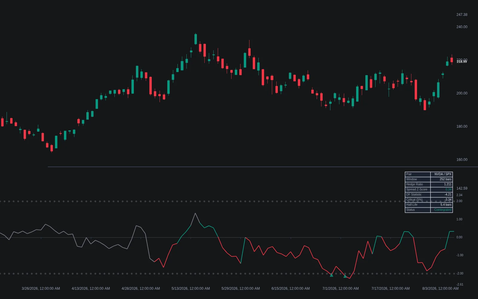
The Engle-Granger procedure tests it: regress one leg on the other and run a Dickey-Fuller test on the residual, comparing the statistic with critical values that account for the estimated hedge ratio. The Johansen test extends the idea to baskets of several instruments. In Python, statsmodels' coint function performs the Engle-Granger test directly. On Quant Charts, the Library's Cointegration indicator does the whole workflow on the chart: a 252-bar rolling regression on log prices against a comparison symbol, the z-scored spread, the test statistic against its critical value, entry events at a z-score of plus or minus two that fire only while the pair tests cointegrated, and a dashboard with the hedge ratio and half-life. The gating matters most: a pair that has stopped testing cointegrated has no reason to revert, and the indicator stands its entries down when that happens. Our pair trading guide covers the strategy from the portfolio side.

Adaptive Hedge Ratios

A hedge ratio estimated over a fixed window lags when the relationship between the legs drifts. The Kalman filter is the standard remedy: it treats the hedge ratio as a hidden state that evolves over time and updates the estimate with each new observation, weighting new information by how noisy the measurement is believed to be. The result is a spread built on a hedge ratio that adapts continuously rather than in jumps at each window boundary, at the cost of two tuning parameters, the assumed process and measurement noise, that materially change behaviour. Ernest Chan's Algorithmic Trading is the accessible reference for the trading application, and the filter itself is well documented.

A Complete Python Backtest

The strategy below fades a z-score beyond two against a 20-day mean, exits when the z-score crosses back through zero, fills on the next bar, and pays a cost on every change of position. It is deliberately the simplest honest version: a loop that tracks position state, then vectorised arithmetic for returns and equity.

window, entry_z, cost_per_change = 20, 2.0, 0.0005     # 5 bps per position change

sma = px.rolling(window).mean()
sd  = px.rolling(window).std()
z   = ((px - sma) / sd).fillna(0)

# State machine: enter when stretched, exit when the z-score crosses back through zero.
pos, states = 0, []
for zi in z:
    if pos == 0:
        pos = 1 if zi < -entry_z else (-1 if zi > entry_z else 0)
    elif (pos == 1 and zi >= 0) or (pos == -1 and zi <= 0):
        pos = 0
    states.append(pos)

signal   = pd.Series(states, index=px.index)
position = signal.shift(1).fillna(0)                       # decided on the close, held from the next bar
returns  = px.pct_change().fillna(0)
costs    = cost_per_change * position.diff().abs().fillna(0)
strategy = position * returns - costs
equity   = (1 + strategy).cumprod()

trades   = int((position.diff().abs() > 0).sum() / 2)
drawdown = equity / equity.cummax() - 1
print(f"trades {trades}, final equity {equity.iloc[-1]:.3f}, max drawdown {drawdown.min():.1%}")

Three checks before believing any output. Count the trades: a rule that fired a dozen times in a decade has told you nothing. Look at the worst drawdown and find the period; for a mean reversion rule on an equity index it will be a trend the rule kept fading, which is the argument for the regime filter in the table above. And re-run with the cost doubled; a strategy that trades often and earns a little per trade is the kind that costs erase first. This article quotes no results because they depend on the instrument, the window and the dates, and because a number without those is a claim rather than evidence. Our guide to building a backtesting engine in Python covers what to add when the rule grows.

Pitfalls Specific to Mean Reversion

Pitfall	Why it bites mean reversion in particular	Defence
Fading a trend	The rule enters against the move and adds as it extends; the largest losses come from the strongest trends	Regime filter, time stop, hard position limit, never unlimited averaging
Assuming normality	Plus or minus two is crossed far more often than 5 percent of the time in fat-tailed data	Treat thresholds as tuned parameters and test their stability, not as probabilities
Correlation mistaken for cointegration	A correlated pair's spread can drift for years	Test cointegration on a rolling window and stop trading a pair that fails
Lookahead in the z-score	Using a mean or standard deviation that includes the bar being traded	Compute on closed bars, fill on the next bar, as the code does
Costs on frequent trades	Short half-lives mean many small trades; spread and commission eat the edge	Charge realistic costs and re-run at double
Fitted thresholds	The entry level that maximised the backtest is the one least likely to repeat	Check neighbouring thresholds and an out-of-sample period
Stops at the extreme	A price stop sits exactly where the rule expects reversion to begin	Time stops and volatility-based position limits instead of, or as well as, price stops

The concepts behind these defences, walk-forward analysis and the in-sample and out-of-sample split, are covered in the Library, and backtesting traps lists the general errors every strategy type shares.

Where Quant Charts Fits

Everything above is faster to try on a chart than in a notebook, and Quant Charts is built for that. Describe the rule to Quant: fade a z-score beyond two against a 20-bar mean, exit at the mean, skip entries when the 200-bar average is falling and the trade would be long. Quant writes the strategy in Pine Script and plots it on the active chart; open Code to read the logic, click Run, and the Backtest Summary reports net profit, trade count, win rate, maximum drawdown and profit factor with commission and slippage set in the strategy properties. Raising the slippage until the edge disappears is the cost test from the Python section done as a settings change. For pairs, the Library's Cointegration indicator runs the statistical test and the z-score on the chart, and Bollinger Bands and RSI load in a click. The Making Strategies with Quant guide shows the workflow.

Adding indicators in Quant Charts. Cointegration, Bollinger Bands and RSI load from the Library; Quant writes the mean reversion rule from a description.

One boundary. The LuxAlgo platform does not place orders for you; Quant Charts is where the rule is written and tested, and execution stays with your broker or your own code, for example through our open-source Trade Relay and Broker SDK.

Conclusion

Mean reversion works when the series being traded genuinely reverts, and fails, often badly, when a trader assumes reversion that is not there. The discipline is to construct a deviation with a stable mean, test it, measure its half-life, express the rule in z-scores so it transfers across instruments, and defend the position against the trends that will eventually come with filters, time stops and limits rather than with hope. Pairs trading applies the same logic to a spread and adds a cointegration test that must keep passing. Prototype the rule on Quant Charts, where Quant writes the Pine Script and the Cointegration indicator runs the statistics, then build it in code once the Backtest Summary says it deserves the effort.

Key Takeaways

Deviations revert; prices do not. Trade the gap to a mean or a cointegrated spread, never a raw price.
Test, then measure the half-life. ADF or KPSS for stationarity; an AR(1) fit for reversion speed; both in statsmodels.
Z-score everything. Bollinger Bands, spreads and oscillator extremes are one rule with unitless thresholds; fat tails make plus or minus two less rare than theory says.
Defend against trends. Regime filter, time stop, position limit, costs charged on every change.
Cointegration for pairs. Correlation is not enough; the Library's Cointegration indicator gates entries on a passing test, and Quant writes the rest.

FAQs

What is a mean reversion strategy?

A rule that trades against a stretched deviation, expecting it to return towards its average: buying when price sits far below a moving average or a spread is unusually wide, selling when the opposite holds, and exiting when the deviation closes. It relies on the deviation having a stable mean, which is a statistical property to test rather than assume.

How do I test whether a market is mean-reverting?

Build the deviation you intend to trade, such as price minus a moving average or a hedge-ratio spread, and run a stationarity test on it: the augmented Dickey-Fuller test, where a small p-value indicates reversion, read alongside KPSS or a variance-ratio test. Then fit an AR(1) model to estimate the half-life; if it is long relative to your horizon, the reversion is too slow to trade profitably after costs.

Are Bollinger Bands and z-scores the same thing?

Yes in substance. Bollinger Bands mark the prices where the z-score of price against its 20-bar mean equals plus or minus two standard deviations. The z-score simply expresses the same deviation as a number, which makes thresholds comparable across instruments and lets the same rule be applied to spreads and oscillators.

What is the difference between correlation and cointegration in pairs trading?

Correlation measures whether two instruments' returns move together bar to bar. Cointegration means some weighted combination of their prices stays anchored to a stable level over time, which is what makes a spread revert. Correlated pairs can drift apart for years; only cointegrated pairs give a spread worth fading, and the relationship can break, so the test should be repeated on a rolling window.

Why do mean reversion strategies lose money in trends?

Because the rule enters against the move and the deviation keeps growing. Market data is fat-tailed, so a z-score beyond two is far more common than the normal distribution suggests and can persist for as long as the trend lasts. The defences are a regime filter that skips trades against a strong trend, a time stop, a hard position limit, and never adding to a loser without a cap.

Can I build and test mean reversion rules on Quant Charts?

Yes. Describe the rule to Quant, for example fade a z-score beyond two against a 20-bar mean and exit at the mean, and Quant writes it in Pine Script; read it in Code, click Run, and the Backtest Summary reports the result with commission and slippage. The Library's Cointegration indicator runs the pairs test and z-score on the chart. The LuxAlgo platform does not place orders for you, so execution stays with your broker.