Python for Trading: Essential Finance Code
Python is useful for trading research because it connects data analysis, indicators, charts and reproducible strategy tests. Its main advantage is a flexible ecosystem and readable code. It is not inherently faster than Java or JavaScript, and choosing Python does not make a strategy profitable.
This guide follows one workflow: validate single-symbol daily bars, calculate moving averages, simulate a long-only rule at the next bar’s open, and review performance with costs included. It then explains optional indicator libraries, backtesting frameworks, broker integration and a complementary research workflow in LuxAlgo.
Example scope: the core pandas/NumPy functions below were tested with synthetic data using pandas 2.2.3 and NumPy 2.3.5. Network downloads, optional TA-Lib calls and broker integrations were not executed. The simulation is educational: it does not model spreads, slippage, partial fills, dividends or borrowing, and it sends no orders.
Set Up a Reproducible Python Environment
Create a virtual environment for the project. Use the same interpreter for installation and execution; on systems where the command is python3, substitute it consistently. These commands create an isolated environment and install the core libraries:
python -m venv trading_env
# macOS/Linux:
source trading_env/bin/activate
# Windows Command Prompt instead:
# trading_env\Scripts\activate.bat
python -m pip install numpy pandas
python -m pip freeze > requirements.txt
Record the Python version, dependency versions, input-data snapshot and strategy settings with each result. A requirements file records the environment; it does not by itself prove compatibility on another operating system.
| Task | Library or tool | What to check |
|---|---|---|
| Numerical arrays | NumPy | Array shape, finite values and units |
| Time-series tables | pandas | Index order, duplicates and missing values |
| Research downloads | yfinance | Adjustment settings, column structure and permitted data use |
| Indicators | TA-Lib | Platform installation, parameters and warm-up |
| Visualization | Matplotlib or Plotly | Time alignment and explicit labels |
| Event-based testing | Backtesting.py or Backtrader | Choose one framework and its documented API |
| Machine learning | scikit-learn | Chronological evaluation and training-only preprocessing |
Install optional libraries only when needed. TA-Lib’s Python wrapper documentation describes binary wheels that include the underlying C library on supported platforms. Start with python -m pip install TA-Lib; use its current source-build instructions if a matching wheel is unavailable. Avoid copying an old platform-specific source archive command into a new environment.
Download Data With Explicit Assumptions
A research download is not a guaranteed execution feed. Check licensing, instrument coverage, adjustment policies, delay, timezone and retention before choosing Yahoo-derived data, Alpha Vantage, Twelve Data or a broker feed. Free access alone does not establish suitability for live trading.
The current yfinance download reference documents automatic OHLC adjustment and multi-level columns as defaults. The following single-symbol example explicitly requests flat, unadjusted columns and retains missing rows for inspection. The end date is exclusive. Install yfinance separately before running it; the network request is not part of the tested offline example.
import yfinance as yf

raw = yf.download(
    "AAPL", start="2024-01-01", end="2025-02-25",
    interval="1d", auto_adjust=False,
    multi_level_index=False, actions=True,
    keepna=True, progress=False,
)
if raw is None or raw.empty:
    raise RuntimeError("No data returned; investigate before testing")
Do not mix unadjusted opens with adjusted closes. Splits and dividends require a coherent price and cash-flow policy; the small simulator below does not implement corporate actions. Use its synthetic example first, or supply a separately validated dataset without such events. Keep dividend and split columns in the raw archive even though the validator selects only OHLCV fields.
Validate Before Calculating Returns
Repeated prices on different dates are valid observations. A blanket drop_duplicates() can erase them. Duplicate timestamps, missing bars and inconsistent ranges need investigation; automatically forward-filling all columns can manufacture prices or volume. This validator rejects questionable inputs rather than silently repairing them.
import numpy as np
import pandas as pd

def prepare_market_data(raw):
    required = ['Open', 'High', 'Low', 'Close', 'Volume']
    if not isinstance(raw, pd.DataFrame) or raw.empty:
        raise ValueError('Expected a nonempty DataFrame')
    if isinstance(raw.columns, pd.MultiIndex) or not raw.columns.is_unique:
        raise ValueError('Select one symbol with unique, flat columns first')
    if not set(required).issubset(raw.columns):
        raise ValueError('Missing OHLCV columns')
    if not isinstance(raw.index, pd.DatetimeIndex):
        raise ValueError('Expected a DatetimeIndex')
    if raw.index.hasnans or not raw.index.is_unique:
        raise ValueError('Missing or duplicate timestamps require investigation')
    if not raw.index.is_monotonic_increasing:
        raise ValueError('Bars must be in chronological order')
    data = raw[required].copy()
    if any(pd.api.types.is_bool_dtype(data[c]) for c in required):
        raise ValueError('Boolean OHLCV values are invalid')
    data = data.apply(pd.to_numeric, errors='raise').astype(float)
    if not np.isfinite(data.to_numpy()).all():
        raise ValueError('Missing or non-finite OHLCV values')
    if (data[['Open', 'High', 'Low', 'Close']] <= 0).any().any():
        raise ValueError('This example requires positive prices')
    if (data['Volume'] < 0).any():
        raise ValueError('Volume cannot be negative')
    if ((data['High'] < data[['Open', 'Close', 'Low']].max(axis=1)) |
        (data['Low'] > data[['Open', 'Close', 'High']].min(axis=1))).any():
        raise ValueError('Inconsistent OHLC ranges')
    data['Returns'] = data['Close'].pct_change(fill_method=None)
    data['Log_Returns'] = np.log(data['Close'] / data['Close'].shift(1))
    return data
This helper assumes positive prices and one symbol. It does not cover instruments that can trade at zero or below, nor does it detect every missing exchange session. Compare the index with the relevant calendar and check that the final bar is complete. Preserve raw data separately; create output folders before writing CSV files. HDF5 storage needs its own optional dependency and format checks.
Calculate Indicators and Explicit Trading Targets
A moving average uses observations available through the current bar. Leave the warm-up undefined until the requested window exists. Here the rule holds one unit when the fast average is above the slow average and otherwise holds cash. It is a target-state rule, not a separate buy order on every bullish bar.
def sma_signals(data, fast=20, slow=50):
    if type(fast) is not int or type(slow) is not int or not 0 < fast < slow:
        raise ValueError('Use integer windows with 0 < fast < slow')
    result = data.copy()
    result['Fast'] = result['Close'].rolling(fast, min_periods=fast).mean()
    result['Slow'] = result['Close'].rolling(slow, min_periods=slow).mean()
    # NaN warm-up stays flat; target 1 means one unit, not 100% of capital.
    result['Target'] = (result['Fast'] > result['Slow']).astype(int)
    return result
The default windows are 20 and 50 bars. They are illustrative settings, not optimized recommendations. A 50/200 comparison answers a different question and requires more history. Keep parameters fixed before evaluating later untouched data.
Optional TA-Lib Indicators
After installing TA-Lib, its documented array API can calculate MACD, RSI and Bollinger Bands. Use the validated close series and explicit parameters. This optional snippet is source-reviewed, not execution-tested here:
import talib

close = data["Close"].to_numpy(dtype=float)
macd, signal, histogram = talib.MACD(
    close, fastperiod=12, slowperiod=26, signalperiod=9
)
rsi = talib.RSI(close, timeperiod=14)
upper, middle, lower = talib.BBANDS(
    close, timeperiod=20, nbdevup=2, nbdevdn=2
)
Set data = prepare_market_data(raw) first. Indicator lookback is function-specific; do not replace initial NaNs with invented values. TA-Lib also documents different propagation of missing inputs from pandas rolling calculations. Compare outputs only when input prices, seeds, parameters and warm-up match.
Chart the Same Data You Tested
A chart function should receive the arrays it plots instead of reading unrelated global variables. Plot prices and moving averages together, then place momentum indicators in a separate panel. Label whether prices are adjusted and use the same timestamps for every series. Matplotlib supports static output; Plotly supports interactive inspection. A visually attractive overlay is not evidence of predictive value.
Simulate Next-Open Execution and Costs
At each completed close, calculate the desired position. Execute that target at the following open. The loop below makes the timing and cash ledger visible: buys subtract price plus a fixed fee, sells add price minus the fee, and equity includes the marked value of any open unit.
def simulate_one_unit(raw, fast=20, slow=50, cash=10000.0, fee=0.10):
    """Completed-close target fills at NEXT open; no broker connection."""
    if not np.isfinite([cash, fee]).all() or cash <= 0 or fee < 0:
        raise ValueError('Invalid cash or per-order fee')
    data = sma_signals(prepare_market_data(raw), fast, slow)
    position, pending = 0, 0
    equity, fills = [float(cash)], []
    for timestamp, row in data.iterrows():
        delta = pending - position
        if delta:
            price = row['Open']
            if delta > 0 and cash < price + fee:
                raise ValueError('Insufficient cash for one unit plus fee')
            cash -= delta * price + fee
            position = pending
            fills.append((timestamp, int(delta), float(price), fee))
        equity.append(float(cash + position * row['Close']))
        pending = int(row['Target'])
    # Last target cannot execute without another bar. Open holdings are marked,
    # not forcibly liquidated; no exit fee is charged until an exit occurs.
    return np.asarray(equity), fills, position
This model assumes sufficient liquidity for one unit at the quoted open. It excludes spread, market impact, latency and rejected orders; add suitable models before relying on real-market results. A fee of $0.10 is a hypothetical per-order input. An open final position is marked at the last close, with no fabricated exit or exit fee.
Run a Small, Reproducible Example
close = np.array([10, 9, 8, 10, 12, 11, 8, 7, 10, 12], dtype=float)
opened = np.array([10, 10, 9, 8, 10, 12, 11, 8, 7, 10], dtype=float)
bars = pd.DataFrame({
    "Open": opened,
    "High": np.maximum(opened, close) + 1,
    "Low": np.minimum(opened, close) - 1,
    "Close": close, "Volume": 100,
}, index=pd.date_range("2025-01-01", periods=10))
equity, fills, position = simulate_one_unit(
    bars, fast=2, slow=3, cash=1000, fee=0.10
)
print(fills)
print(round(equity[-1], 2), position)
These are artificial daily observations, not an exchange calendar or market dataset. The example buys at $12 on the sixth bar, sells at $8 on the eighth, and buys at $10 on the tenth. Three $0.10 fees leave $997.70 of marked equity and one unit open. It demonstrates mechanics, not an investment result.
Move to a Framework Deliberately
Backtesting.py’s API uses Backtest and Strategy; Backtrader is a different package with a different API. Install and follow the framework you actually use. For a long-only Backtesting.py strategy, use self.position.close() for an exit; a generic self.sell() can create an opposite position instead.
Check order size, commissions on entry and exit, next-open versus close execution, indicator warm-up and the handling of final open trades. Integer size 1 means one unit; a fraction below one represents a share of available liquidity. Those are not interchangeable. Reconcile a small known ledger before comparing a framework result with your own simulator.
Measure Performance Without Universal Pass Marks
Include starting equity in the running peak so an immediate loss is counted as drawdown. Handle undefined ratios explicitly. This helper assumes positive equity and equally spaced observations; its Sharpe calculation uses a zero risk-free rate and a configurable annualization factor.
def equity_metrics(equity, periods_per_year=252):
    values = np.asarray(equity, dtype=float)
    if values.ndim != 1 or len(values) < 2:
        raise ValueError('Include starting equity and at least one later value')
    if not np.isfinite(values).all() or (values <= 0).any():
        raise ValueError('This helper requires finite, positive equity')
    if not np.isfinite(periods_per_year) or periods_per_year <= 0:
        raise ValueError('Invalid annualization factor')
    returns = values[1:] / values[:-1] - 1
    volatility = returns.std(ddof=1) if len(returns) > 1 else np.nan
    sharpe = (returns.mean() / volatility * np.sqrt(periods_per_year)
              if np.isfinite(volatility) and volatility > 1e-12 else np.nan)
    drawdowns = values / np.maximum.accumulate(values) - 1
    return {'Return': values[-1] / values[0] - 1,
            'Max Drawdown': float(drawdowns.min()),
            'Sharpe (zero risk-free rate)': float(sharpe)}
For ordinary daily equity observations, 252 is a common annualization convention; it is not appropriate for every market or irregular series. Use an aligned risk-free return series for excess-return analysis. Constant returns or a single observation do not support the Sharpe estimate used here. Serial correlation and small samples also limit interpretation.
| Metric | Interpretation | Review alongside |
|---|---|---|
| Return | Change in marked equity including modeled costs | Exposure, benchmark and holding period |
| Maximum drawdown | Largest decline from an earlier equity peak | Duration, recovery and stress scenarios |
| Sharpe ratio | Mean return relative to variability under stated assumptions | Sample length, serial dependence and risk-free convention |
| Win rate | Fraction of closed trades with a profit | Average win/loss and costs |
| Profit factor | Gross closed-trade profit divided by gross loss | Trade count and undefined denominator when no losses occur |
There is no universal Sharpe, drawdown, win-rate or profit-factor threshold that makes a strategy deployable. Separate training and evaluation periods, document every parameter search, and test sensitivity to costs. For machine learning, fit preprocessing only on training data and apply it to later observations without refitting on the evaluation set.
Treat Broker Automation as a Separate System
A successful offline test does not establish a safe broker connection. The Interactive Brokers TWS API documentation is the reference for the installed API version, callbacks, connection settings and order state. Use a deliberate paper-account configuration and verify the actual account; a familiar port number alone is not proof of paper mode.
- Wait for connection readiness and synchronize order identifiers before submission.
- Validate instrument identity, quantity, side, price constraints and aggregate exposure, including working orders.
- Track acknowledgments, partial fills, rejects and cancellations separately from submitted intent.
- After a timeout or restart, reconcile broker state before retrying an uncertain order.
- Keep credentials out of source files and logs; restrict access and define recovery procedures.
- Define stop-new-orders, cancel-orders and close-position actions separately.
Python can automate a rule, but it cannot remove judgment from strategy selection, deployment or intervention. Event loops, concurrency and callback signatures require integration tests with the actual broker environment. The examples here do not connect to an account or place trades.
Use LuxAlgo Alongside Python Research
Begin with LuxAlgo’s native charts to inspect market structure and compare related setups. Keep the symbol, timeframe, source and adjustment assumptions consistent when comparing chart observations with Python data.
Ask Quant, our coding agent to implement a precise strategy specification. Inspect the generated code and run it yourself. Check signal timing, position size, warm-up and costs before interpreting the results. A chart strategy and a Python simulator need matched assumptions before their outputs can be compared.
Example prompt: “Create a long-only 20/50 moving-average strategy. Explain completed-bar signals, entry and exit timing, position sizing and fees, and identify every assumption I must match in a separate Python test.”
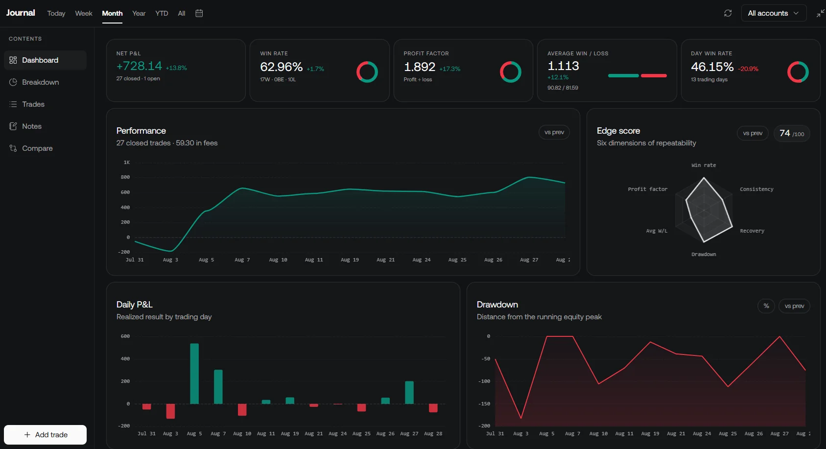
Review compatible recorded trade files in the native journal. Keep simulated trades distinct from recorded executions and reconcile any differences in costs, timestamps or quantities.
For developer integrations, review the current documentation and supported interfaces of each tool. Exporting values between languages requires explicit schema, timestamp and numerical checks; matching an indicator name alone does not guarantee matching outputs. Avoid assuming a private Python API or universal cross-platform parity.
Python Trading Video and Further Practice
The original QuantProgram beginner tutorial, published January 14, 2022, covers setup, Python concepts, strategy testing and API workflows. It is an older course: use the current library references above for installation and API details, and treat demonstrations as learning examples rather than a ready-to-deploy system.
Start with the synthetic ledger, then add one feature at a time: a documented data source, realistic costs, a benchmark and untouched evaluation data. Preserve the inputs and results so a change can be explained. Profile actual bottlenecks before changing languages or adding complexity.
Frequently Asked Questions
Is Python fast enough for trading?
Python is useful for research and many automated workflows, especially with numerical libraries. Execution speed depends on the workload, implementation and infrastructure; measure the actual bottleneck rather than assuming a language-wide speed advantage.
Why can yfinance code fail when selecting Close or Adj Close?
Download settings affect adjusted prices and column structure. Specify the adjustment policy and single-symbol column format explicitly, inspect the returned data, and handle empty or missing results before calculating indicators.
Should I forward-fill every missing market-data value?
No. Missing prices, volume and sessions have different meanings. Preserve the original data, investigate gaps and apply a documented field-specific policy rather than fabricating complete bars.
How does the example avoid same-bar execution bias?
It computes a target after the completed close and executes that target at the following open. The final target is not executed without another bar, and any open position is marked at the final close.
Can LuxAlgo replace testing a Python trading system?
LuxAlgo charts, Quant and the journal support research and review. Inspect generated code and run it yourself, then separately validate Python calculations, fill assumptions, broker integration and operational controls.
Read next