Risk Parity Allocation with Python

Risk parity allocates a portfolio by risk rather than by capital: each asset is sized so that it contributes the same share of the portfolio's volatility, which usually means far less equity and far more bonds than a conventional 60/40 mix. The idea was developed at Bridgewater Associates, whose All Weather strategy launched in 1996 and which the firm describes as the foundation of the risk parity movement. In Python the whole method fits in a few dozen lines: a covariance matrix, a function that measures each asset's risk contribution, and an optimizer that equalizes those contributions. This guide builds it step by step, with a worked example you can check by hand, a walk-forward backtest that avoids the usual lookahead, a cost model, the pitfalls that turn a tidy backtest into a disappointing live portfolio, and how to monitor each sleeve on Quant Charts, where Quant, our coding agent, can write the weight dashboard for you.
Key points:
- Risk contribution is the unit. An asset's contribution is its weight times its marginal risk; the contributions sum to portfolio volatility, so equalizing them is a well-defined target.
- Inverse volatility is the special case. Weighting each asset by one over its volatility gives equal risk contributions only when all pairwise correlations are equal; otherwise you need the optimizer.
- Backtest on completed windows. Estimate covariance from bars that had closed before the rebalance date, then hold the weights until the next one.
- Unlevered risk parity is low-volatility by construction. Its return in equity bull markets trails 60/40; institutions add leverage to match a volatility target, which brings its own risks.
What Risk Parity Means
A 60/40 portfolio holds 60 percent of its capital in stocks, but because stocks are several times more volatile than government bonds, nearly all of its risk comes from the equity sleeve. Risk parity fixes that imbalance by asking a different question: not how much money goes into each asset, but how much of the portfolio's variance each asset is responsible for. The equal risk contribution (ERC) portfolio is the allocation where every asset answers with the same number.
Two consequences follow. First, an unlevered ERC portfolio of stocks and bonds is dominated in capital terms by bonds, so its expected return is lower than 60/40 and its volatility much lower. Institutional risk parity funds typically lever the portfolio up to a target volatility, which is why the approach is sometimes described as levered bonds. Second, the allocation depends entirely on the covariance matrix: change the estimation window and the weights change, and when correlations shift, as they did in 2022 when stocks and bonds fell together, the diversification the method assumes weakens.
The Mathematics
Let w be the vector of weights and Σ the covariance matrix of returns. Portfolio variance is wᵀΣw and volatility σₚ is its square root. The marginal contribution of asset i is the partial derivative of σₚ with respect to wᵢ, which equals (Σw)ᵢ divided by σₚ. Multiplying by the weight gives the total risk contribution:
RC_i = w_i * (Σ w)_i / σ_p
sum over i of RC_i = σ_p            # contributions add up to portfolio volatility
ERC target: RC_i = σ_p / n          # every asset carries 1/n of the risk
Because the contributions sum to σₚ, the share of risk carried by each asset is RCᵢ divided by σₚ, and the ERC portfolio is the one where every share equals one over n. When all correlations are equal, the solution is weights proportional to one over each asset's volatility, the naive or inverse-volatility risk parity. With unequal correlations the closed form disappears and a numerical solver takes over.
A Worked Example You Can Check
Take two uncorrelated assets: stocks with 16 percent annual volatility and bonds with 4 percent. With zero correlation, portfolio variance is the sum of the squared weighted volatilities, so the numbers below are exact.
| Allocation | Stock variance term | Bond variance term | Portfolio volatility | Share of risk (stocks / bonds) |
|---|---|---|---|---|
| 60 / 40 by capital | 0.36 × 0.0256 = 0.009216 | 0.16 × 0.0016 = 0.000256 | 9.73% | 97.3% / 2.7% |
| 20 / 80 by capital (ERC) | 0.04 × 0.0256 = 0.001024 | 0.64 × 0.0016 = 0.001024 | 4.53% | 50% / 50% |
The 60/40 portfolio is, in risk terms, a stock portfolio with a small bond position attached. The 20/80 portfolio balances the two, and it does so with less than half the volatility, which is the property risk parity is prized for and the reason its unlevered return is lower. The weights are exactly inverse to volatility, 1/16 against 1/4, because the correlation was zero. Add a positive correlation and the optimizer below will shift the balance.
Setting Up in Python
The implementation needs NumPy and pandas for the arithmetic, SciPy for the optimizer, yfinance for data, and Matplotlib for charts. Riskfolio-Lib, a portfolio optimization library built on CVXPY, is optional and provides a tested risk parity solver with many risk measures.
pip install numpy pandas scipy yfinance matplotlib riskfolio-libData
Recent versions of yfinance adjust prices for splits and dividends by default, so the adjusted series is in the Close column; set the flag explicitly so the code does not depend on a default. Convert to simple daily returns and drop the first row.
import numpy as np
import pandas as pd
import yfinance as yf

tickers = ["SPY", "TLT", "GLD"]            # US equities, long Treasuries, gold
prices = yf.download(tickers, start="2010-01-01", end="2025-01-01",
                     auto_adjust=True, progress=False)["Close"]
prices = prices.dropna(how="any")          # keep dates where every asset traded
returns = prices.pct_change().dropna()
print(returns.tail())
Dropping dates where any asset is missing keeps the covariance matrix honest; forward-filling a stale price into a day the market moved understates that asset's volatility and its correlation with the others. If the assets trade on different calendars, align on the intersection of dates or resample to weekly returns.
Building the Risk Parity Solver
Risk Contributions
def portfolio_volatility(weights, cov):
    return float(np.sqrt(weights @ cov @ weights))

def risk_contributions(weights, cov):
    sigma = portfolio_volatility(weights, cov)
    marginal = cov @ weights                 # d sigma / d w, times sigma
    return weights * marginal / sigma        # sums to sigma

cov = returns.cov().values * 252             # annualised covariance
w_6040 = np.array([0.6, 0.4, 0.0])
rc = risk_contributions(w_6040, cov)
print("volatility:", round(portfolio_volatility(w_6040, cov), 4))
print("risk shares:", np.round(rc / rc.sum(), 3))
Run this on the real data and the equity sleeve's share will be far above its capital weight, the same pattern as the worked example. That printout is the diagnostic to keep: any allocation method can be judged by the risk shares it produces.
The Equal Risk Contribution Optimizer
The objective is the sum of squared differences between each asset's risk contribution and the average contribution. It is zero exactly at the ERC solution. Constrain the weights to sum to one and bound each between zero and one, so the portfolio is long only and unlevered, and use SLSQP, which handles both constraint types.
from scipy.optimize import minimize

def erc_objective(weights, cov):
    rc = risk_contributions(weights, cov)
    target = rc.mean()
    return float(np.sum((rc - target) ** 2)) * 1e4   # scaled for the solver

def erc_weights(cov):
    n = cov.shape[0]
    start = np.repeat(1.0 / n, n)
    constraints = ({"type": "eq", "fun": lambda w: np.sum(w) - 1.0},)
    bounds = [(0.0, 1.0)] * n
    result = minimize(erc_objective, start, args=(cov,), method="SLSQP",
                      bounds=bounds, constraints=constraints,
                      options={"ftol": 1e-12, "maxiter": 500})
    if not result.success:
        raise RuntimeError(result.message)
    return result.x

w_erc = erc_weights(cov)
rc_erc = risk_contributions(w_erc, cov)
print("weights:", dict(zip(tickers, np.round(w_erc, 3))))
print("risk shares:", np.round(rc_erc / rc_erc.sum(), 3))   # about 1/3 each
Check the output before trusting it: the three risk shares should be equal to several decimal places and the weights should be highest for the lowest-volatility asset. If the solver reports failure, the covariance matrix is usually the culprit, either because two assets are nearly identical or because the window is too short for the number of assets.
The Riskfolio-Lib Alternative
Riskfolio-Lib solves the same problem as a convex program and supports risk measures beyond variance. Its Portfolio object takes the returns DataFrame, estimates the statistics, and the rp_optimization method returns the risk parity weights. The default risk budget is equal across assets; pass a vector to the b argument to set unequal budgets.
import riskfolio as rp

port = rp.Portfolio(returns=returns)
port.assets_stats(method_mu="hist", method_cov="hist")
w_rp = port.rp_optimization(model="Classic", rm="MV", rf=0, b=None, hist=True)
print(w_rp.T.round(3))
Compare its weights with those from the SLSQP solver; with the same covariance estimate they should agree closely. Changing rm to a downside measure such as CVaR produces a different portfolio, because it balances tail risk rather than variance.
Backtesting Without Lookahead
A Walk-Forward Loop
The rule is simple to state and easy to break: on each rebalance date, estimate covariance from the window of returns that ended the previous day, solve for weights, and apply those weights to the returns that follow. The loop below rebalances on the first trading day of each month, uses a one-year window, and charges a transaction cost proportional to turnover.
def backtest_erc(returns, lookback=252, cost_bps=5.0):
    months = returns.index.to_period("M")
    weights = None
    daily = []
    for i in range(lookback, len(returns)):
        new_month = months[i] != months[i - 1]
        if weights is None or new_month:
            window = returns.iloc[i - lookback:i]          # ends yesterday
            new_w = erc_weights(window.cov().values * 252)
            turnover = 0.0 if weights is None else np.abs(new_w - weights).sum()
            weights = new_w
        else:
            turnover = 0.0
        gross = float(weights @ returns.iloc[i].values)
        daily.append(gross - turnover * cost_bps / 1e4)
    return pd.Series(daily, index=returns.index[lookback:], name="ERC")

def backtest_fixed(returns, weights, lookback=252):
    w = np.asarray(weights)
    return pd.Series(returns.iloc[lookback:].values @ w,
                     index=returns.index[lookback:], name="Fixed")

erc = backtest_erc(returns)
sixty_forty = backtest_fixed(returns, [0.6, 0.4, 0.0])
Note what the loop does not do. It does not use the covariance of the month it is about to trade, it does not rebalance on the same bar it estimated on, and it does not ignore the cost of moving from the old weights to the new ones. Those three omissions are the most common ways a risk parity backtest flatters itself.
Measuring the Result
def summarize(series, periods=252):
    growth = (1 + series).cumprod()
    years = len(series) / periods
    cagr = growth.iloc[-1] ** (1 / years) - 1
    vol = series.std() * np.sqrt(periods)
    sharpe = series.mean() / series.std() * np.sqrt(periods)   # risk-free rate 0
    drawdown = growth / growth.cummax() - 1
    return pd.Series({"CAGR": cagr, "Volatility": vol, "Sharpe": sharpe,
                      "Max drawdown": drawdown.min()})

report = pd.concat([summarize(erc), summarize(sixty_forty)], axis=1)
report.columns = ["ERC", "60/40"]
print(report.round(3))
Read the report in this order. Volatility should be much lower for ERC, because that is what the method targets. Compare Sharpe ratios rather than returns, since the two portfolios run at different risk levels. Look at maximum drawdown alongside the period it covers; a table of numbers hides whether the drawdown happened in one crisis or several. Finally, split the sample and confirm the ordering holds in both halves. This article deliberately prints no results of its own: the figures depend on the tickers, the window and the dates, and a number quoted without them is not evidence.
Plotting the Comparison
import matplotlib.pyplot as plt

curves = pd.DataFrame({"ERC": (1 + erc).cumprod(),
                       "60/40": (1 + sixty_forty).cumprod()})
ax = curves.plot(figsize=(11, 5), logy=True, title="Growth of 1 unit")
ax.set_ylabel("Portfolio value (log scale)")
plt.tight_layout()
plt.show()
A log scale is essential here, because the unlevered ERC curve will sit below 60/40 in most equity bull markets and the difference in slope is what matters, not the gap in level. If you want to compare at equal volatility, scale the ERC series by the ratio of the two volatilities before plotting, and remember that doing so in practice means borrowing.
Pitfalls and Practical Choices
| Pitfall | What goes wrong | Mitigation |
|---|---|---|
| Noisy covariance | A one-year window on daily data estimates every correlation with error; weights swing between rebalances and turnover rises | Lengthen the window, shrink the estimate (Ledoit-Wolf in scikit-learn), or limit how far weights may move per rebalance |
| Correlation regime change | The method assumes the assets diversify one another; in 2022 stocks and long bonds fell together and the balance offered little protection | Add sleeves with different drivers, monitor rolling correlations, and size for the possibility that they converge |
| Leverage to reach a return target | Unlevered ERC returns less than 60/40 in equity bull markets; levering it up adds financing cost and forced deleveraging in drawdowns | Decide the volatility target first, model the borrowing cost explicitly, and cap gross exposure |
| Lookahead in the backtest | Estimating covariance through the rebalance day, or trading at the same bar's close, leaks information | End the estimation window the day before, trade at the next open, as the loop above does |
| Ignoring costs | Monthly rebalancing of several ETFs is cheap; the same rule on futures with roll costs or on illiquid assets is not | Charge turnover-proportional costs, and test a tolerance band that rebalances only when weights drift past a threshold |
| Too many assets for the window | With n assets the covariance matrix has n(n+1)/2 parameters; a short window cannot estimate them all | Group similar assets into sleeves and run risk parity across the sleeves |
Rebalancing Bands
A tolerance band is a cheap improvement over calendar rebalancing. Compute the target weights on schedule but trade only when any current weight has drifted from its target by more than a threshold, and when you do trade, move all the way back to target. The code is a few lines and it typically cuts turnover substantially without changing the risk profile much.
def needs_rebalance(current, target, band=0.05):
    return bool(np.any(np.abs(np.asarray(current) - np.asarray(target)) > band))
Monitoring the Sleeves on Quant Charts
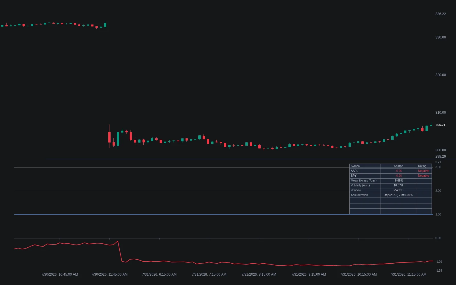
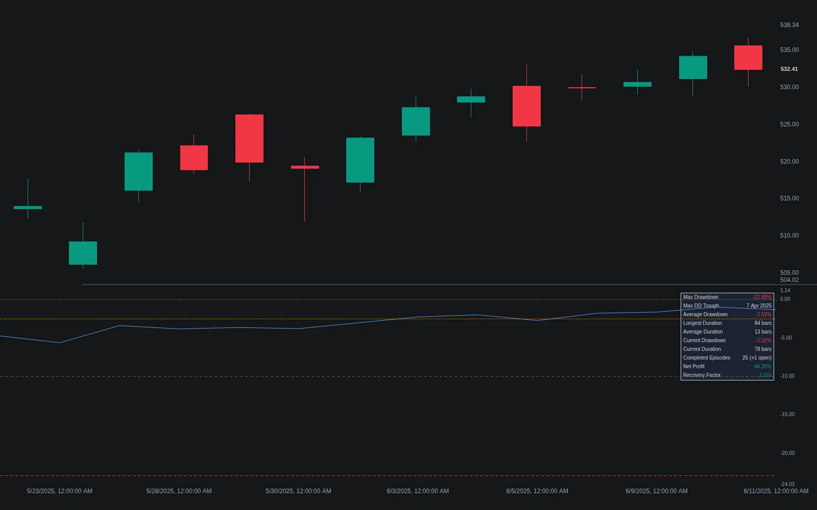
Python builds the allocation; a charting platform is where you watch whether its assumptions still hold. On Quant Charts, the Library's Sharpe Ratio indicator plots a rolling risk-adjusted score for the chart symbol and ranks up to three comparison symbols in a dashboard, so SPY, TLT and GLD can be read on one pane. The Drawdown Statistics indicator profiles each sleeve's declines from peak with depth, duration and recovery, which is the fastest way to see which asset produced the portfolio's worst month. Both are native indicators, added from the Library in a click.
For the allocation itself, describe the rule to Quant: pull the daily closes of the three symbols, compute 60-day volatility for each, and show inverse-volatility weights in a table on the chart. Quant writes the script in Pine Script, plots it on the active chart, and you can open Code to read how it fetched each series before you click Run. Pair the dashboard with a rolling correlation study and the two assumptions risk parity depends on, stable volatilities and diversifying correlations, are visible every day. The Making Strategies with Quant guide covers how Quant also builds testable strategies with a Backtest Summary. Executing the rebalance remains a task for your broker; no LuxAlgo tool places orders.
One boundary worth stating: Library indicators are trading tools, not allocation engines. For the allocation research itself, our guides on hierarchical risk parity, why correlation alone is not enough and building a backtesting engine in Python continue where this one stops.
Conclusion
Risk parity replaces a judgment about how much money to put in each asset with a rule about how much risk each may carry, and Python makes the rule executable: measure the risk contributions, equalize them with an optimizer, re-estimate on a schedule using only the data that was available, and charge yourself for every trade. The method's virtues, low volatility and balanced exposure, are structural and show up in any honest backtest. Its weaknesses, dependence on a noisy covariance estimate and on correlations that can converge in a crisis, are structural too. Build the diagnostics before the allocation, keep the risk-share printout and the drawdown profile in view, and treat any return figure that arrives without its window and dates as a claim rather than a result.
Key Takeaways
- Risk contribution, not capital. RCᵢ = wᵢ(Σw)ᵢ/σₚ; the contributions sum to portfolio volatility and ERC sets them equal.
- Inverse volatility is only exact with equal correlations. Use the SLSQP solver or Riskfolio-Lib's rp_optimization otherwise.
- Estimate on completed data, trade after. The walk-forward loop ends its window the day before each rebalance and charges turnover.
- Expect lower returns unlevered. Compare on Sharpe ratio and drawdown, and model leverage cost explicitly if you scale up.
- Monitor the assumptions. Sharpe Ratio and Drawdown Statistics on Quant Charts, and a Quant-written inverse-volatility dashboard, keep them in view.
FAQs
What is risk parity allocation?
Risk parity sizes each asset so that it contributes an equal share of the portfolio's total volatility, rather than an equal or fixed share of capital. Because low-volatility assets such as government bonds need larger weights to carry the same risk as equities, an unlevered risk parity portfolio holds far more bonds than a 60/40 mix and runs at much lower volatility.
How is risk contribution calculated?
With weights w and covariance matrix Σ, portfolio volatility is the square root of wᵀΣw. Asset i's risk contribution is wᵢ times (Σw)ᵢ divided by portfolio volatility. The contributions sum to the portfolio's volatility, so each asset's share is its contribution divided by that total. The NumPy implementation is three lines and is the diagnostic to run on any allocation.
Is inverse-volatility weighting the same as risk parity?
Only when every pair of assets has the same correlation. In that case weights proportional to one over each asset's volatility produce equal risk contributions exactly, as in the two-asset zero-correlation example in this article. With unequal correlations the equal-risk-contribution weights must be found numerically, with SciPy's SLSQP or a library such as Riskfolio-Lib.
Why does risk parity often return less than 60/40?
Because it is a low-volatility portfolio. Balancing risk across stocks and bonds means holding mostly bonds, so in periods when equities rally the unlevered portfolio lags. Institutional implementations lever the portfolio to a volatility target to close the gap, which adds financing cost and the risk of forced selling in drawdowns. Compare the two on Sharpe ratio and drawdown rather than raw return.
How do I avoid lookahead in a risk parity backtest?
Estimate the covariance matrix from a window that ends the day before the rebalance, apply the new weights to the returns that follow, and charge a cost proportional to the change in weights. Never include the month you are about to trade in the estimation window, and do not trade at the close of the bar you estimated on. The backtest loop in this article follows those rules.
Can I monitor a risk parity portfolio on Quant Charts?
Yes. The Library's Sharpe Ratio indicator plots a rolling risk-adjusted score with a dashboard for comparison symbols, and Drawdown Statistics profiles each sleeve's declines. Quant can write a Pine Script that fetches several symbols, computes rolling volatility and displays inverse-volatility weights in a table; inspect it in Code and click Run. Trades are placed at your broker, not by any LuxAlgo tool.
References
LuxAlgo Resources
- Quant Charts
- LuxAlgo Quant
- Making Strategies with Quant
- Sharpe Ratio Indicator
- Drawdown Statistics Indicator
- Sharpe Ratio Concept
- Drawdown Statistics Concept
- Correlation Concept
- Hierarchical Risk Parity Rebalancing Methods
- Top Tools for Risk Parity Optimization
- Portfolio Correlation Is Not Enough
- How to Build a Backtesting Engine in Python
- Maximum Drawdown: Calculation and Use Cases
- Walk-Forward Testing vs Backtesting
External Resources
Read next