The Key to Understanding RSI (Relative Strength Index)
The Relative Strength Index (RSI) compares smoothed positive and negative price changes and expresses their balance on a 0–100 scale. It measures momentum in the selected price series. It does not estimate intrinsic value, prove that an asset is cheap or expensive, or guarantee a reversal.
Developed by J. Welles Wilder, RSI is commonly displayed with a 14-period length and reference levels at 70 and 30. This guide explains its calculation, alternative averaging methods, interpretation and derived indicators, including the important implementation details that can make two apparently identical RSI settings disagree.
What Overbought and Oversold Mean Here
“Overbought” and “oversold” describe an oscillator reading relative to chosen thresholds. They are not statements that price lies above or below fundamental value. RSI can remain elevated during an advance or depressed during a decline. A threshold crossing is an observation from price history, not advance knowledge of the next move.
Use the interval as part of the definition: 14 daily changes and 14 fifteen-minute changes summarize different horizons. The source series, missing bars, price adjustments, initialization and averaging method also matter.
Calculate Wilder’s RSI
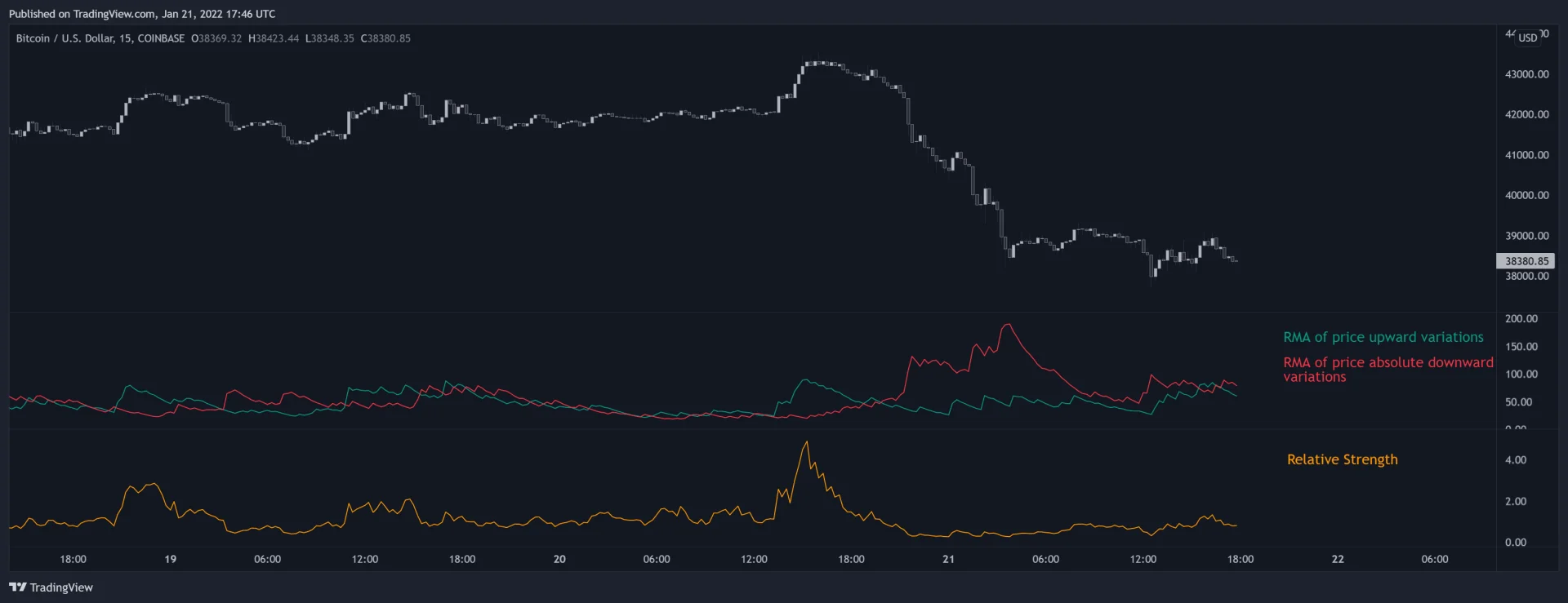
Let Pₜ be the selected closing price and n a positive integer length. Separate each price change into a nonnegative gain and loss, then smooth both with Wilder’s moving average, often called RMA or SMMA.
Δₜ = Pₜ − Pₜ₋₁
uₜ = max(Δₜ, 0)
dₜ = max(−Δₜ, 0)
Gₜ = (1 − 1/n)Gₜ₋₁ + uₜ/n
Lₜ = (1 − 1/n)Lₜ₋₁ + dₜ/n
RS = Gₜ / Lₜ
RSI = 100 − 100/(1 + RS)
A common initialization averages the first n gains and losses before applying the recurrence. Record the convention used by the implementation. Starting both filters at zero or using a different amount of prior history can change early readings.
For Gₜ + Lₜ greater than zero, the same result can be written more directly:
RSI = 100 × Gₜ/(Gₜ + Lₜ)
    = 100 × RMA(u, n)/RMA(|Δ|, n)
The second equality requires the same smoothing and compatible initialization for all terms, because u + d = |Δ|. If the average gain is 2 and average loss is 1, RS is 2 and RSI is about 66.67. That number describes the gain/loss balance under the averaging rule; it is not a 66.67% probability of an upward move.
Handle Zero Denominators Explicitly
| State | Mathematical implication | Implementation check |
|---|---|---|
| G > 0, L = 0 | RSI is 100 using the gain-over-total form | Avoid dividing by zero while computing RS |
| G = 0, L > 0 | RSI is 0 | Keep the loss magnitude nonnegative |
| G = 0, L = 0 | The ratio is undefined | Specify missing output, a neutral convention or retained state |
| Insufficient history | The selected seed is not ready | Do not silently treat unavailable values as valid signals |
A flat initial price history can produce zero gains and losses even with exponential smoothing. With a finite SMA window, n consecutive zero changes make the total change magnitude zero. RMA and EMA retain decaying past state, but that does not eliminate all flat-start or numerical edge cases. Match the actual platform’s convention when comparing results.
Changing the Average Changes the Indicator
Cutler’s SMA-Based RSI
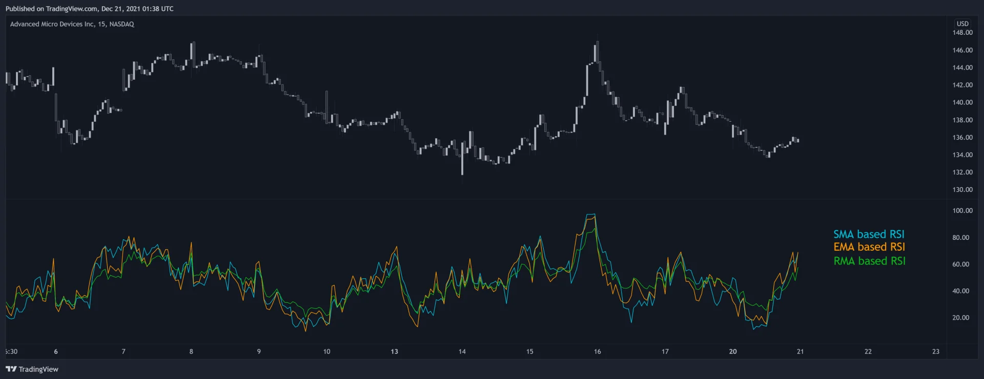
Replacing Wilder smoothing with a simple average gives a finite-window version commonly called Cutler’s RSI. Over n price changes, the signed changes telescope to the difference between the newest and oldest prices:
Cutler RSI = 100 × Σ max(Δᵢ, 0) / Σ |Δᵢ|
           = 50 + 50 × (Pₜ − Pₜ₋ₙ) / Σ |Δᵢ|
Sums cover the n changes ending at t; denominator must be positive.
Equivalently, the signed price difference divided by n can be divided by SMA(|Δ|, n), multiplied by 50 and shifted by 50. A new observation removes the oldest change completely from this window. That can produce abrupt changes when a large old move drops out. It does not mean every SMA-based reading must react sooner than every exponentially smoothed reading.
EMA Versus Wilder Smoothing
A conventional EMA uses α = 2/(m+1), while Wilder smoothing uses α = 1/n. At the same numerical length above 1, the EMA puts more weight on the latest observation. To match the smoothing coefficient, solve:
2/(m+1) = 1/n
m = 2n − 1
Wilder length 14 ↔ EMA length 27
The two recurrences then match only when they receive the same inputs and begin from equal states. A platform that seeds a 27-period EMA differently from a 14-period RMA can still return different values, particularly early in the series.
Length Affects Smoothing, Not a Guaranteed Distribution
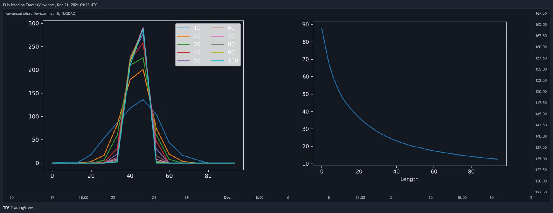
Longer averaging often reduces short-lived fluctuations. In a sample where positive and negative changes are sufficiently balanced, readings may cluster nearer 50. But a persistent sequence of positive changes can produce RSI at 100 regardless of the length once initialized. A sustained imbalance can keep RSI away from its midpoint.
Do not infer that every longer RSI must have a smaller realized range, that all price changes have zero mean, or that a narrower sample distribution makes reversals easier to predict. Those are separate empirical questions. Compare the same instrument and evaluation period, with enough prior history for each setting.
Interpret Levels and the Midpoint as Testable Conditions
Crossing above 70 or below 30, returning inside those levels, and crossing 50 are different events. Define which one is used. A return from an extreme can occur later and at a different price; it does not guarantee that continuation risk has disappeared.
When the denominator is positive, RSI above 50 means smoothed gains exceed smoothed losses. Below 50 means the opposite. This can be used as a momentum filter, but it does not prove the existence or future continuation of a price trend. Repeated midpoint crossings can produce whipsaws.
Triangles, wedges, support/resistance-like levels and other shapes can also be drawn on RSI. Their identification depends on selected turns and scale. They are transformations of the same underlying observations, not independent evidence from a separate market source.
Define Divergence with Corresponding Swings
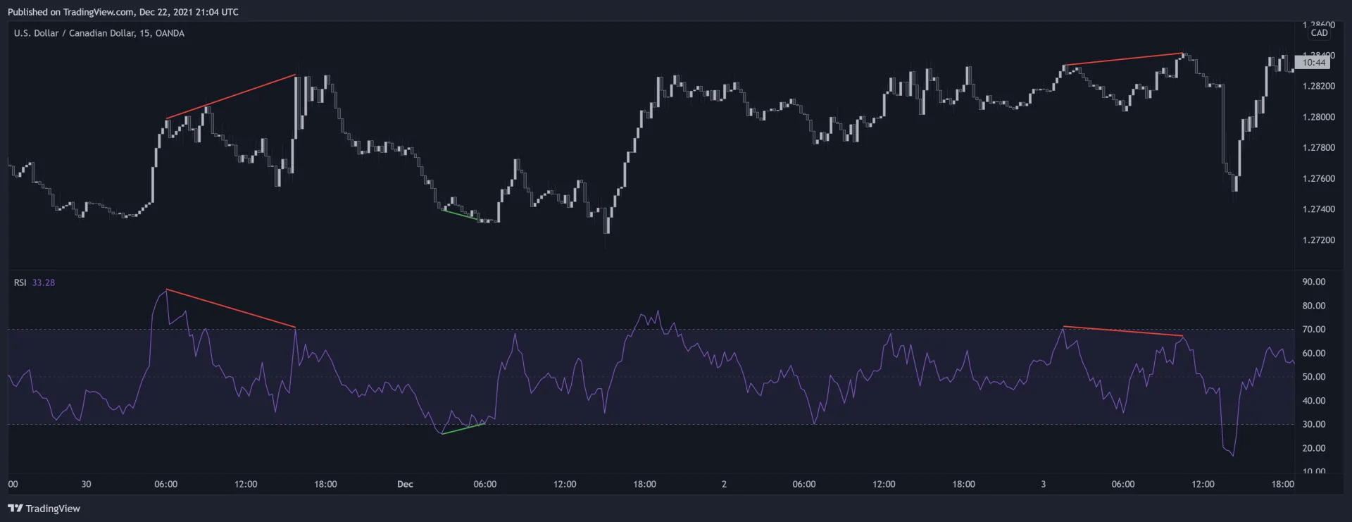
A regular bearish divergence commonly compares a higher price high with a lower RSI high. A regular bullish divergence compares a lower price low with a higher RSI low. Use corresponding swings and specify their confirmation timing. This is more precise than describing divergence as generic negative correlation between the two series.
Divergence can persist while price keeps trending. Its presence alone supplies neither an entry price nor an invalidation rule. If a pivot is recognized only after later bars, preserve that delay in any backtest; plotting the marker back at the turn does not make the information available earlier.
Failure Swings Are an RSI Sequence
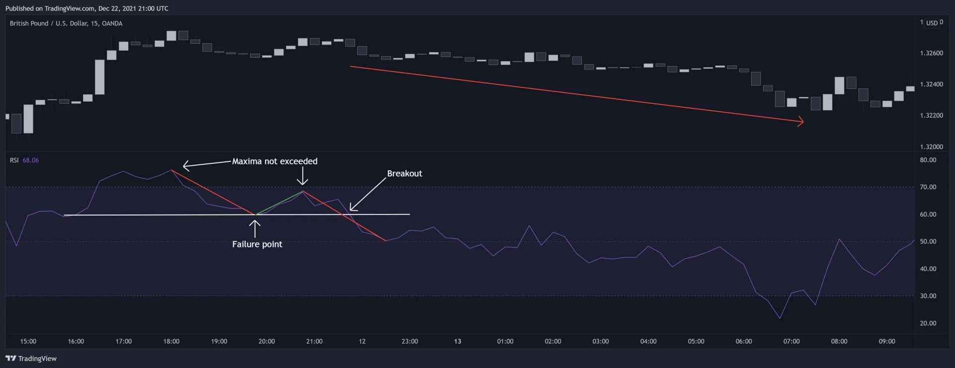
In the bearish version shown, the break of the intervening RSI low completes the sequence. The bullish mirror starts below 30, rebounds, pulls back while holding above 30, then breaks the intervening RSI high. Define the turns and the exact crossing condition before using this as a strategy. A failed attempt to make another extreme does not by itself complete this oscillator sequence.
Correct the Connors Two-Period Setup
Larry Connors’ published RSI research investigates short-horizon returns after extreme two-period readings in a historical stock sample. Those reported averages are not promises for today’s markets, and they do not establish that all 14-period applications are useless.
The documented RSI(2) setup looks for a short-term pullback within the direction of a longer-term filter. The original article reversed that filter. The corrected example is:
| Component | Long-side example | Short-side example |
|---|---|---|
| Trend filter | Price above the 200-day SMA | Price below the 200-day SMA |
| RSI condition | Two-period RSI below 5 | Two-period RSI above 95 |
| Example exit | Price moves above the 5-day SMA | Price moves below the 5-day SMA |
| Still to define | Order timing, costs, sizing and adverse-exit policy | The same, plus short availability and borrowing costs |
A reading below a threshold and a fresh crossing below it are not identical rules. Specify whether entry uses a closing observation, an order before the close or a later open. A test cannot use the final closing value to guarantee a fill before that value was known. Overnight gaps, repeated signals and missed fills also matter.
This is RSI with a two-period length, not the separate composite indicator called ConnorsRSI. A higher chart interval does not automatically remove frictional costs. Evaluate the chosen instrument, holding period and execution assumptions, and do not interpret historical testing without stops as a guarantee against large losses.
Stochastic RSI Measures RSI Within Its Own Range
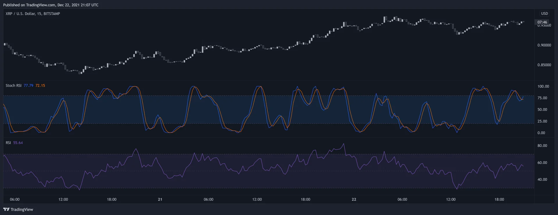
Raw StochRSI = 100 × (RSIₜ − lowest(RSI, k))
                    / (highest(RSI, k) − lowest(RSI, k))
This form is scaled to 0–100 when its denominator is positive; some implementations use 0–1. Displayed %K and %D may add further smoothing. If the highest and lowest RSI are equal, a zero-range policy is required. The transform can amplify small changes in a narrow RSI range, but it does not add future information. Its realized range and distribution still depend on the input, window and smoothing.
Ehlers’ Inverse Fisher Transform
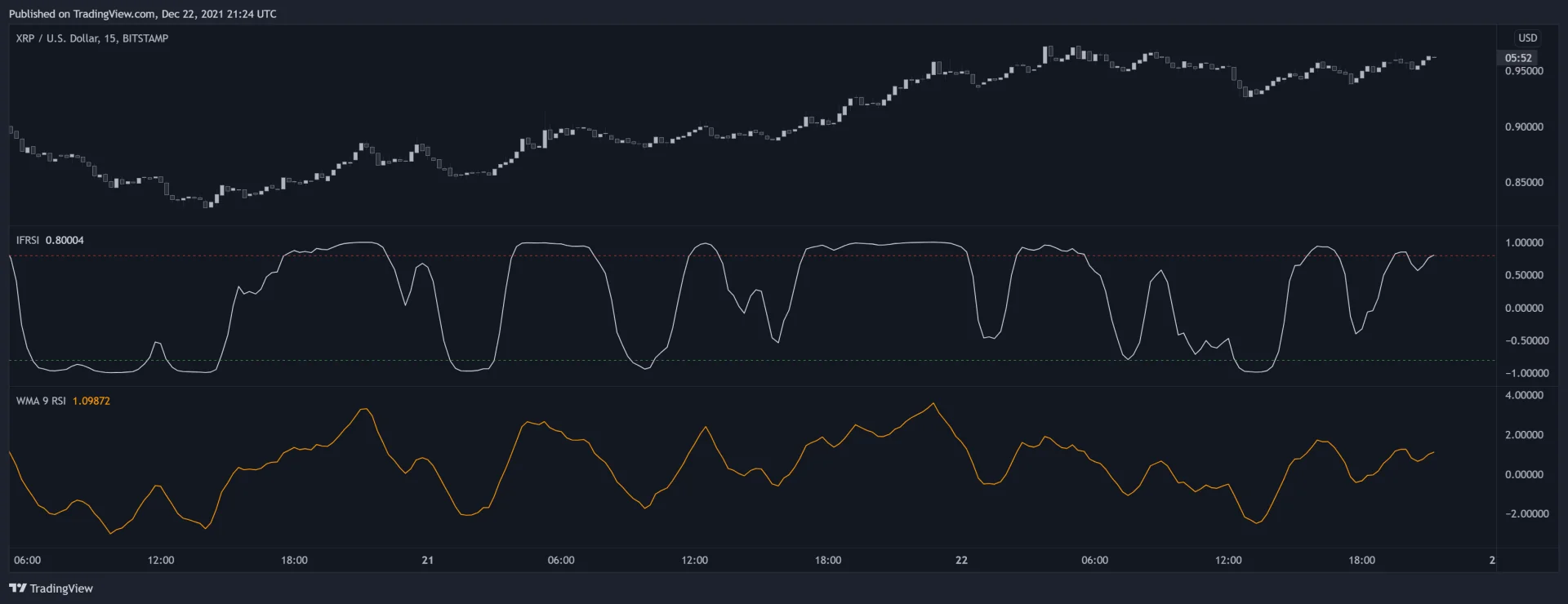
In The Inverse Fisher Transform, John Ehlers gives this specific sequence: a five-period RSI, rescaling, a nine-period weighted moving average, then the inverse Fisher function.
vₜ = 0.1 × (RSI(P, 5) − 50)
zₜ = WMA(v, 9)
IFisherₜ = (exp(2zₜ) − 1)/(exp(2zₜ) + 1)
         = tanh(zₜ)
The function compresses finite inputs into the open interval (−1, 1). A numerically stable tanh implementation avoids unnecessary exponential overflow. Whether observations cluster near the bounds depends on the input distribution and scaling; a U-shaped distribution is not guaranteed. A sharply switching display is not proof of accurate or profitable signals.
Laguerre RSI Uses Filter Stages Rather Than Ordinary RSI as Input
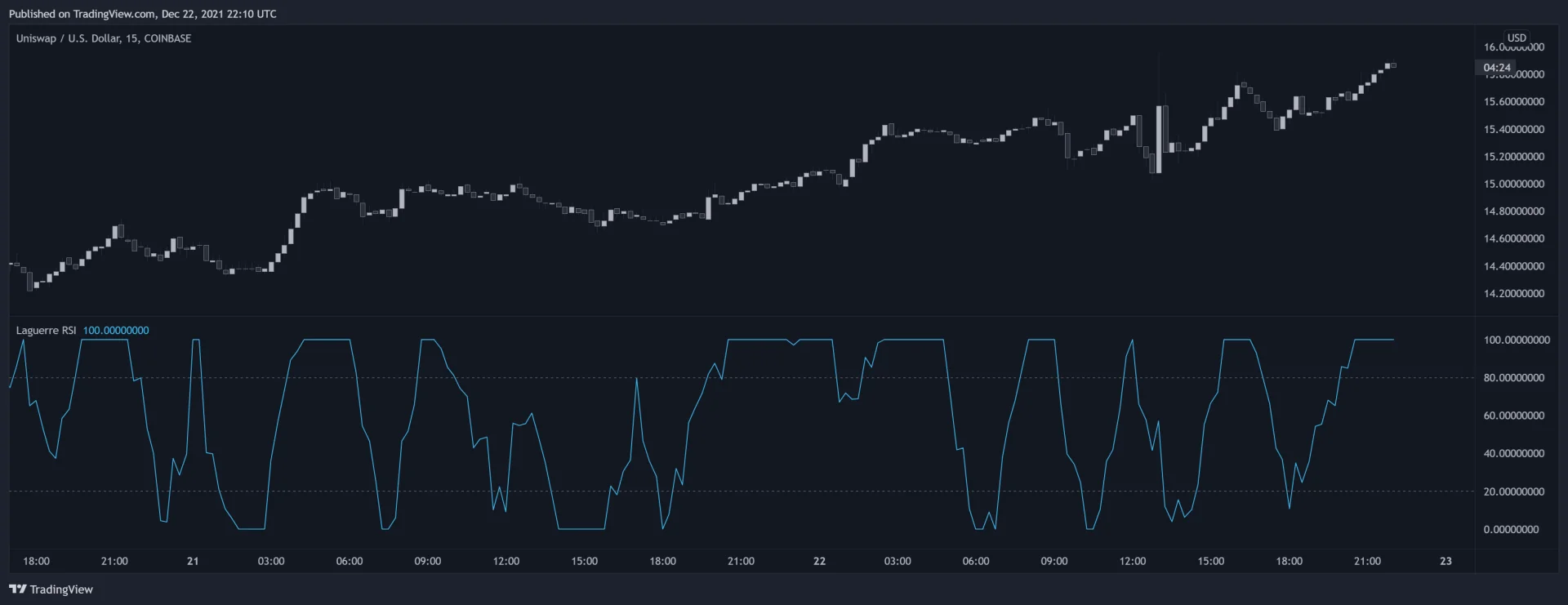
Ehlers’ Time Warp—Without Space Travel constructs four recursive stages. Bracket [1] below means the previous bar’s value; calculate the current stages in order. A usual smoothing parameter satisfies 0 ≤ γ < 1, with values nearer 1 placing more persistence in the filter.
L0 = (1 − γ) × P + γ × L0[1]
L1 = −γ × L0 + L0[1] + γ × L1[1]
L2 = −γ × L1 + L1[1] + γ × L2[1]
L3 = −γ × L2 + L2[1] + γ × L3[1]
q0 = L0 − L1; q1 = L1 − L2; q2 = L2 − L3
CU = max(q0,0) + max(q1,0) + max(q2,0)
CD = max(−q0,0) + max(−q1,0) + max(−q2,0)
Laguerre RSI = 100 × CU/(CU + CD), when CU + CD > 0
The signed-difference form in the original article is algebraically equivalent on the same states:
num = q0 + q1 + q2
den = |q0| + |q1| + |q2|
Laguerre RSI = 50 + 50 × num/den, when den > 0
The paper’s code displays the unscaled 0–1 ratio, starts its states at zero and updates the ratio only when CU + CD is nonzero. A 0–100 display multiplies that result by 100. Preserve or explicitly document initialization and the zero-denominator policy. Changes to γ affect the recursion, but neither a U-shaped distribution nor a particular prediction lead follows automatically.
Test the Implementation in LuxAlgo’s Native Charts
Use LuxAlgo’s native charts to fix the symbol, interval, input series, seed convention and variant before comparing signals. Keep development data separate from a later evaluation period. Review standard price candles and realistic costs when turning indicator conditions into trading rules.
Ask Quant, our coding agent to express a supported hypothesis with the exact formula, threshold timing, exits and sizing. Inspect the generated code and run it manually. Review strategy settings and individual trades rather than judging the method only by the shape of the oscillator.
Check native data coverage and history. The documented US-equity source is Cboe EDGX rather than a consolidated all-venue feed. Re-run the test after changing symbols, intervals or assumptions.
Frequently Asked Questions
Does overbought RSI mean price is above intrinsic value?
No. It means the oscillator is above a selected threshold. RSI measures the balance of price changes, not fundamental value.
Is EMA-based RSI with length 27 identical to Wilder RSI with length 14?
Their smoothing coefficients match. Exact outputs also require the same inputs and equal initial states; different seeding conventions can produce differences.
Can RSI calculations divide by zero?
Yes. A flat initial series or a finite window of zero changes can leave the denominator at zero. Implementations need an explicit policy for that case.
What is the corrected Connors RSI(2) trend filter?
The documented example looks for long opportunities above the 200-day SMA and short opportunities below it, combined with short-term RSI extremes and defined exits.
Do RSI variants reliably predict reversals?
No. They transform observed prices in different ways. A useful trading rule still requires explicit timing, costs, risk controls and evaluation on later data.
Read next